What is an LSTM?

Dependencies in sequential input. Because LSTMs include feedback connections, they may handle complete data sequences instead of just individual data points, which is different from standard neural networks. This enables ideas to remain, much as how people comprehend words in an essay by referring to earlier words rather than beginning at the beginning.
The powerful Long Short-Term Memory (LSTM) unit overcomes many obstacles in training recurrent neural networks (RNNs), particularly learning long-term dependencies.
The Problem LSTMs Address: Vanishing and Exploding Gradients
When learning long-term dependencies, when knowledge from far-off previous time steps is essential for precise predictions in the present, traditional Recurrent Neural Networks frequently encounter major difficulties. The vanishing gradient problem and, less frequently, the expanding gradient problem are the main causes of this difficulty.
Vanishing Gradient: As the gradients propagate over several layers or time steps during training, they may get smaller and smaller, guiding the model’s learning. Information from the distant past becomes nearly meaningless as a result, making it challenging for the network to learn and modify the weights of previous layers.
Exploding Gradient: On the other hand, gradients may occasionally become unnecessarily big, which might result in inconsistent learning and unpredictable model updates.
By guaranteeing a constant gradient flow where mistakes retain their value, LSTMs are specifically built to address these issues and enable them to capture long-term connections in data efficiently.
Architecture of LSTM

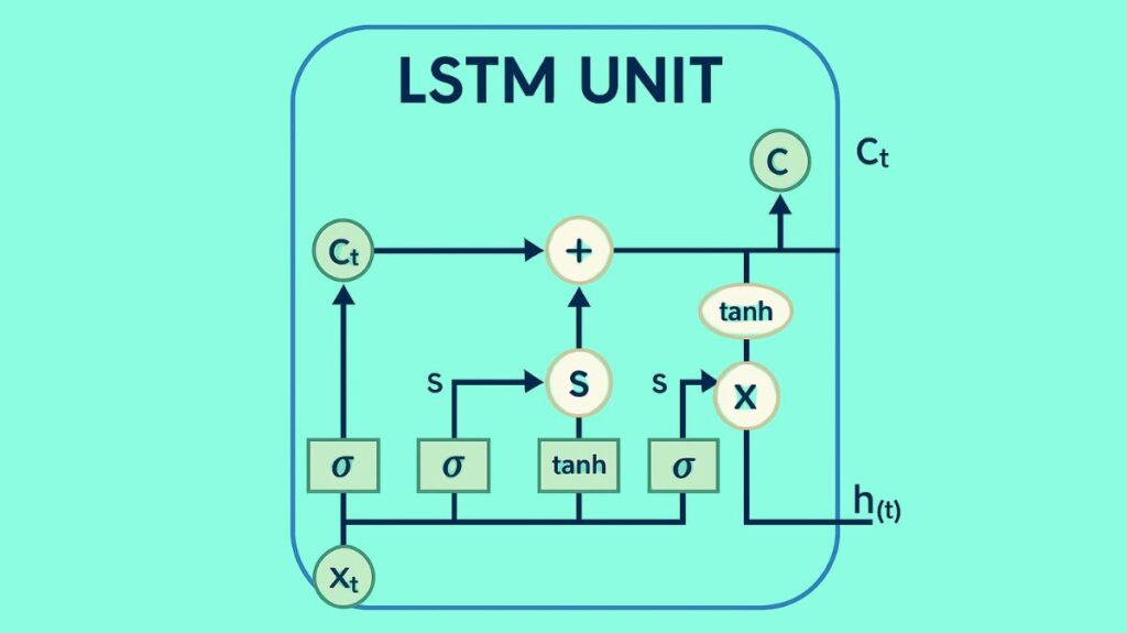
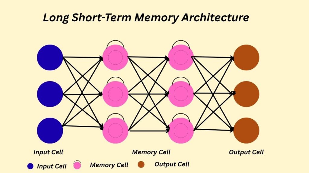
An LSTM’s distinct memory cell (or cell state) and gating mechanisms are the foundation of its efficacy.
Memory Cell: The memory cell preserves a state across time by serving as a long-term memory storage device. It is thought of as a “conveyor belt” that passes directly across the network’s whole chain, allowing information to move along it almost unaltered with just slight linear exchanges. Information from dozens or even hundreds of previous time steps can be stored in this cell.
Gates: The forget gate, input gate (sometimes called the write gate), and output gate are the three different kinds of gates used in LSTMs. In essence, these gates are constructions that selectively let information to flow through. They consist of a pointwise multiplication operation and a layer of sigmoid neural networks. By producing values between 0 and 1, where 0 denotes “let nothing through” and 1 denotes “let everything through,” the sigmoid layer controls the information flow.
There are four interacting layers or neural networks that make up an LSTM unit (or “cell”). LSTMs have a hidden state, which is essentially their short-term memory, in addition to their cell state.
Detailed Breakdown of LSTM Gates with Examples
These gates are used in a sequence of stages that the LSTM uses to process information:
Forget Gate ((f_t))
Purpose: Because it is no longer helpful, this gate decides which data from the previous cell state ((C_{t-1})) should be ignored or lost.
Mechanism: It requires the prior hidden state ((h_{t-1})) and the current input ((x_t)). These are run via a sigmoid function, which gives each value in the cell state a number between 0 and 1. The prior cell state is then multiplied element-by-element by this output.
Example: Consider the following sentence: “Bob is a nice person. Dan, on the other hand, is evil.” This is what a language model would analyze. When the model reaches the full stop and begins discussing “Dan,” the forget gate will choose to remove the data about “Bob” from its memory cell, allowing the data about “Dan” to be used.
Input Gate ((i_t)) and New Information ((\hat{C}_t))
Purpose: The new information from the current input that is relevant and has to be added or saved in the cell state is determined in this stage.
Mechanism: There are two components to this:
- The “input gate layer” or sigmoid layer determines which particular input values need to be changed.
- With values ranging from -1 to 1, a tanh layer generates a vector of new candidate values ((\hat{C}_t)) that could be added to the state.
- The additional information that will be included into the cell state is then created by combining these two components through element-wise multiplication.
Cell State Update: Prior to adding the new, pertinent information (multiplying (i_t) with (\hat{C}t)), the old cell state ((C_{t-1})) is updated into the new cell state ((C_t)) by first “forgetting” the bits that are not important (multiplying by (f_t)). (C_t = f_t \o. C{t-1} + i_t \o. \hat{C}_t) is the formula for this update.
- Example: The statement “Bob knows swimming” comes to mind. He informed me on the phone that he had spent four arduous years in the military. The input gate would classify the detail about “over the phone” as less important in this situation, while identifying “served the navy for four long years” as crucial new knowledge about Bob that has to be added to the cell state.
Output Gate ((o_t))
Purpose: This gate determines whether data from the updated cell state ((C_t)) will be utilized to calculate the LSTM unit’s current hidden state (output). A filtered representation of the cell state is the output.
Mechanism: In order to identify the portions of the cell state that are pertinent for output, a sigmoid layer first analyses the input ((x_t)) and the prior hidden state ((h_{t-1})). Second, a tanh activation function is applied to the cell state in order to scale its values from -1 to 1. The filtered output, which is the hidden state ((h_t)) for the current time step, is then obtained by multiplying these two results element-wise.
Example: For the phrase “Bob fought the enemy alone and gave his life for his nation.” After the model encountered the term “brave,” the output gate would filter the cell state to output information relevant to a person (such as “hero”) because Bob is the “brave” entity.
These gates let LSTMs learn and use long-term dependencies by selectively storing or dismissing information as it travels through the network.
Bidirectional LSTMs
The Bidirectional LSTM (Bi-LSTM) is a noteworthy variation. Bi-LSTMs process input data concurrently in both forward and backward directions, in contrast to regular LSTMs, which only process information from the past to the future. The input sequence is trained on two different LSTM layers one on the regular input sequence and the other on the inverted input sequence to accomplish this.
For applications that demand a thorough comprehension of the complete input sequence, this bidirectional processing capacity can greatly enhance performance by enabling the network to extract context from both historical and future data inside a time series. Bi-LSTMs, for example, have demonstrated better performance and resilience in COVID-19 prediction when compared to other models and regular LSTMs.
Core Mechanism: Constant Error Carousel (CEC)
LSTM’s Constant Error Carousel is its main invention. A center linear unit with a fixed self-connection (weight 1.0) in a memory cell represents this. This fixed self-connection prevents the vanishing or inflating gradient problem by allowing error signals held in the memory cell to flow back indefinitely without being magnified exponentially.
Applications of LSTM
Because they can manage sequential data and long-term dependencies, LSTMs are effective tools in deep learning and artificial intelligence that are employed in many different applications:
Natural Language Processing (NLP)
- Predicting the subsequent word in a series is known as language modelling.
- Machine translation is the process of translating text across languages.
- Condensing lengthy texts or producing grammatically sound phrases are examples of text generation and summarization.
- Sentiment Analysis: Identifying the text’s emotional tone.
- Named Entity Recognition (NER): Recognizing and categorizing text’s named entities.
Speech Recognition and Synthesis: Recognizing instructions, producing voice, and translating spoken language into text.
Time Series Analysis and Forecasting: Estimating future values like stock prices, weather trends, or energy usage by using historical data.
Audio and Video Data Analysis: Convolutional Neural Networks are frequently used in conjunction with object detection, activity recognition, and action categorization in movies.
Handwriting Recognition and Generation: Making sense of and producing handwritten text.
Anomaly Detection: Finding odd data patterns that can be used to detect fraud or network infiltration.
Recommender Systems: Making recommendations for books, music, or films based on user activity patterns.
Bioinformatics: Including drug design, protein homology detection, and protein secondary structure prediction.
Medical Image Analysis: Frequently used in combination with CNNs for tasks like MRI image categorization and brain tumor detection.
COVID-19 Applications: For COVID-19 detection, diagnosis, classification, prediction, and forecasting, several researchers have employed LSTM-based models, which have demonstrated good accuracy in a number of investigations.
Advantages and Limitations of LSTM
Advantages:
- LSTM solves tasks with minimal time lags over 1000 steps; older approaches struggle even with lower lags (e.g., 10 steps).
- Handles noise, scattered inputs, and accurate continuous values without considerable degradation over time.
- LSTM can extract temporal order information from widely spaced inputs.
- LSTM demonstrates good generalization, outperforming typical LSTMs on longer sequences.
- LSTM can function as a controller network in Neural Turing Machines (NTMs), which connect neural networks with external memory resources. LSTM controllers learn faster and generalize better than feedforward controllers or normal LSTM networks on copying, repeat copy, and associative recall, especially for longer sequences.
Limitations:
- The efficient trimmed backprop variant of LSTM may struggle with “strongly delayed XOR problems” or tasks where completing subgoals does not steadily reduce error.
- Increased Parameters: Memory cell blocks may require more input and output gates, potentially raising weights by up to a factor of 9 compared to standard recurrent nets completely connected.
- Parity Problems: LSTM’s behavior may be similar to feedforward networks, making it unsuitable for 500-step parity problems that can be solved faster by random weight guessing.
- LSTM may struggle with counting discrete time steps if extremely minor temporal variations are important, similar to other gradient-based techniques.
Accelerating LSTMs with GPUs
The parallel processing capabilities of GPUs (Graphics Processing Units) can greatly reduce the computational burden of training and inference procedures for LSTMs. Due to their significant speedups such as a 6x speedup during training and a 140x greater throughput during inference when compared to CPU implementations GPUs have emerged as the de facto standard for LSTM utilization. LSTM recurrent neural network training and inference on GPUs is especially supported by libraries such as cuDNN and TensorRT, which are components of the NVIDIA Deep Learning SDK.
Finally, because of their special memory cells and gating methods, LSTMs successfully address the long-term reliance issue, marking a major breakthrough in recurrent neural networks. As a result, they are now essential for a variety of sequence learning and prediction problems in many fields.
