Types Of Restricted Boltzmann Machine
Restricted Boltzmann Machines (RBMs) come in two types, each intended to process a certain type of data. The probability distribution applied to their visible (input) and hidden units is the main way in which these types differ from one another. those are namely:
- Binary Restricted Boltzmann Machine
- Gaussian Restricted Boltzmann Machine
Binary Restricted Boltzmann Machine (RBM)
Binary Restricted generative stochastic neural networks are fundamentally based on Restricted Boltzmann Machine (RBM). They are made to model data utilizing binary variables for both their input and hidden units. For activities involving binary data, like text, where the existence of words can be represented as 1s and 0s, or black-and-white graphics, where pixels are either on or off, they are especially well-suited.
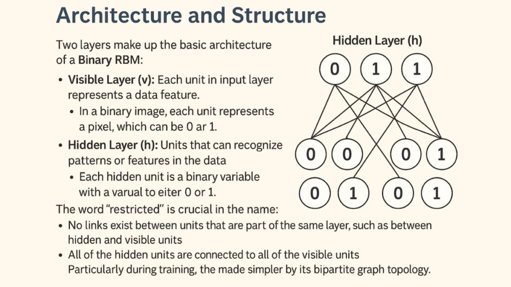
Binary Restricted Boltzmann Machine Architecture and Structure

Two layers make up the basic architecture of a Binary RBM:
Visible Layer (v): Each unit in the input layer represents a data feature. Each unit in a binary image represents a pixel, which can be 0 or 1.
Hidden Layer (h): Units that can recognize patterns or features in the data make up this layer. Additionally, every hidden unit is a binary variable that can have a value of either 0 or 1.
The word “restricted” is crucial in the name:
- No links exist between units that are part of the same layer, such as between hidden and visible units.
- All of the hidden units are connected to all of the visible units.
Particularly during training, the model’s calculations are made simpler by its bipartite graph topology.
Core Mechanism: Learning and Reconstruction
Finding the underlying probability distribution of the input data is the primary objective of a Binary RBM. It does this by modifying weights and biases to favour particular visible and hidden unit configurations.
Training: The original input data is reconstructed by the network during training. It learns the weights that enable it to respond to an input pattern by activating certain hidden units, and then it uses those active hidden units to precisely replicate the original input pattern.
Gibbs Sampling: The model updates the states of its units iteratively. Using an input as a starting point, it probabilistically activates the hidden units. A new visible layer is then rebuilt using the activated hidden units. The network can identify a stable configuration that accurately represents the data thanks to this back-and-forth procedure, which is called Gibbs sampling.
Purpose and Applications
Binary RBMs are mostly employed in:
Generative Modeling: After being trained, an RBM can be used to produce fresh data that resembles the training set. The network will eventually generate new samples that represent the patterns it discovered by initializing the visible or hidden layer with a random configuration and then executing the Gibbs sampling procedure.
Feature Extraction: One could think of a trained RBM’s hidden layer as a potent feature extractor. The hidden layer’s activation patterns provide a condensed, insightful depiction of the input data. This makes them ideal for pre-training deep neural networks in an unsupervised manner, after which the learnt features are transferred to a supervised classifier.
Collaborative Filtering: Recommendation systems can be constructed using binary RBM. In this case, the hidden units might stand in for user preferences or traits, while the visible units might represent objects (like movies). The RBM learns to anticipate a user’s preferences based on their past behaviour.
To put it simply, a Binary RBM is a basic component of Deep Learning that integrates the ideas of generative modelling and Unsupervised Learning to learn and represent data in a condensed and probabilistic manner.
Gaussian Restricted Boltzmann Machine (RBM)

In the context of modelling continuous data, such as sensor or audio signals, input and hidden units are Gaussian-distributed continuous variables.
Architecture and Unit States
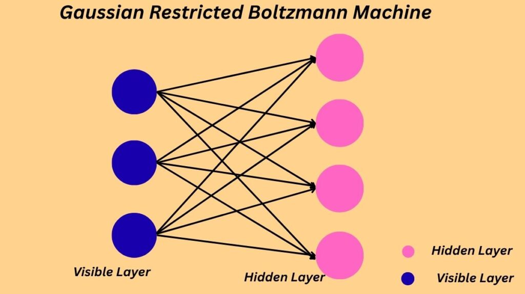
Restricted Boltzmann Machines (RBMs) that are specifically made to handle continuous, real-valued input data are known as Gaussian RBMs. Its visible units are the primary distinction from a Binary RBM.
Visible Layer: The visible layer’s units are continuous and can have any actual value. A Gaussian distribution is used to simulate when a visible unit is activated. This enables the model to work immediately without the requirement for discretization with raw data, such as pixel intensities (0-255), temperature readings, or audio signal amplitudes.
Hidden Layer: The Gaussian-Bernoulli RBM is a more popular and potent variation, even though your statement implies that both layers are continuous. Because the hidden units in this architecture are still binary (0 or 1), the model is compelled to learn a binary, sparse representation of the continuous input data. This mix of binary hidden units and continuous visible units works very well for feature extraction.
Core Mechanism and Training
By minimizing an energy function, a Gaussian RBM learns a probability distribution across the data, which is the same basic idea as a binary RBM. This process’s specifics are modified for continuous variables, though.
Energy Function: For a Gaussian RBM, the variance of the visible units is represented by a term in the energy function. The RBM learns the ideal variance for every visible unit during training in order to best predict the data, in addition to the weights and biases.
Training and Activation: To deal with the continuous units, the training algorithm usually Contrastive Divergence is adjusted.
- Forward Pass: The sigmoid function still determines the likelihood of a hidden unit being triggered, as in a Binary RBM.
- Backward Pass: An alternative activation function is employed to recreate the visible units. A Gaussian distribution whose mean is the weighted sum of the states of the hidden units is used to sample the state of a visible unit.
Specific Applications
The advantage of Gaussian RBMs in many real-world situations is their direct modelling of continuous data.
Audio and Signal Processing: Audio spectrograms are continuous arrays of frequencies and amplitudes that can be used to identify patterns. Gaussian RBMs can also be used to model raw time-series data from sensors. This can be applied to tasks such as feature extraction and signal denoising.
Natural Image Processing: Greyscale images (with pixel values ranging from 0 to 255) and, with some architectural enhancements, color images can be modelled using Gaussian RBMs, in contrast to Binary RBMs, which are restricted to black-and-white images. Low-level elements like borders and texturing are easily learnt by them.
Dimensionality Reduction: A Gaussian RBM can be utilized as a potent tool for dimensionality reduction on continuous datasets by learning a compressed representation in the hidden layer. This allows the model to efficiently capture the most significant characteristics in a lower-dimensional space.
Financial Data: Model time-series data such exchange rates, stock prices, and other financial indicators for trend analysis and anomaly detection.
