What is Backpropagation Through Time?

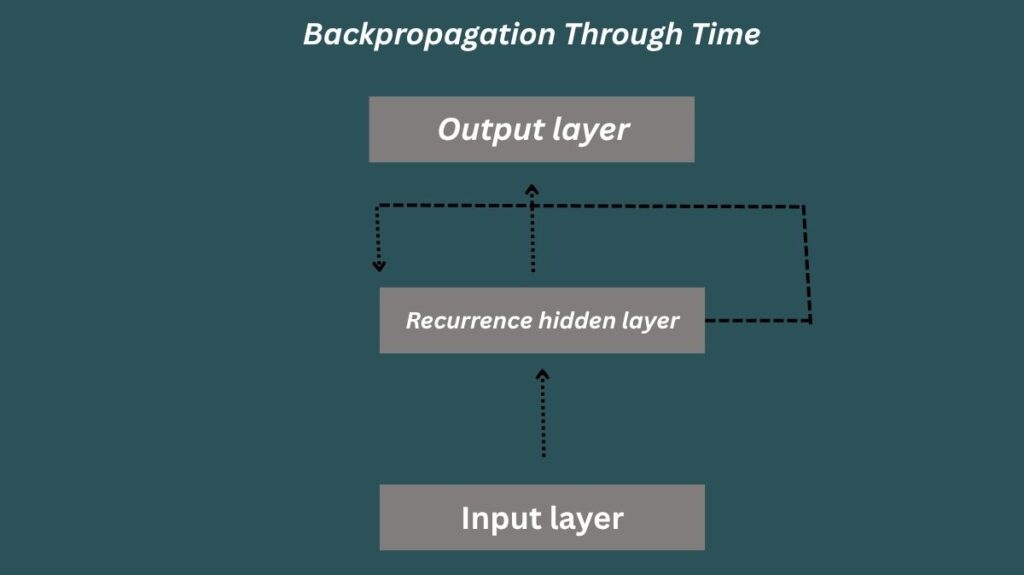
Backpropagation Through Time (BPTT) is a technique created especially for Recurrent Neural Network (RNN) training. RNNs analyze sequential data, which means that using a “memory” element, their outputs are impacted by both the current input and past inputs, in contrast to traditional neural networks whose outputs are solely dependent on the current input. With the help of this memory, RNNs may identify temporal connections in language or time series data.
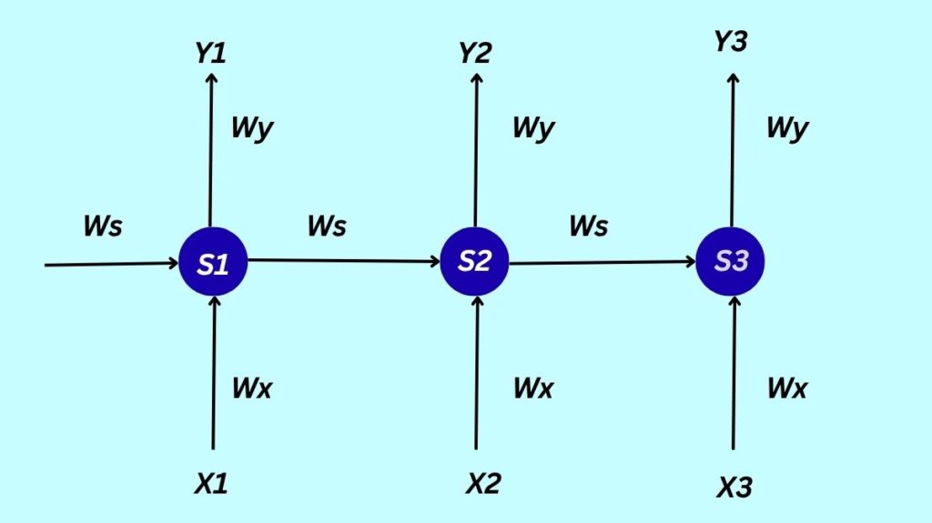
By essentially “unfolding” the network over time, BPTT goes beyond conventional backpropagation protocols. The RNN at a given time step is represented by each “layer” in the resulting network of interconnected feedforward networks. Importantly, the weights in this unfolded structure are the same for all time steps, which reflects the original RNN’s recurrent character. This makes it possible for RNNs to pick up intricate temporal patterns.
RNN Architecture

The hidden state (S_t or h_t) that an RNN maintains at each time step t serves as the network’s memory, accumulating data from earlier inputs. By merging the current input (X_t) and the prior hidden state (S_{t-1}), the hidden state S_t is updated. Non-linearity is then introduced by applying an activation function. This hidden state is then transformed to provide the output (Y_t or \^{y}_t).
The output and hidden state can be expressed mathematically as follows:
- St=g1(WxXt+WsSt−1)
- The formula Y_t = g_2(W_y S_t) has activation functions g_1, g_2 (or \ϕ_h, \ϕ_o) and weight matrices W_x, W_s, and W_y for inputs, hidden states (recurrent connections), and outputs, respectively. Interestingly, there are fewer parameters because the same weight matrices are employed at each time step.
Mechanism of BPTT
There are various steps involved in the BPTT training process:
Unfolding the RNN: The network is theoretically stretched out across time, as previously stated, producing a unique “copy” of the RNN for every time step.
Forward Pass: Through this unfolded network, the input sequence is fed. The hidden state from the previous time step and the current input are used to calculate the activations and outputs at each time step.
Backward Pass (Backpropagation): A function for errors, such as squared error E_t = (d_t – Y_t)^2) calculates the difference between the desired output (d_t) and the projected output (Y_t). After then, this defect is backpropagated from the final time step backwards to the beginning time step throughout the unfolding network. To calculate the gradients of the loss with respect to the weights and biases of the network, the chain rule is utilized. Since weights are shared over time steps, the total gradient for each shared weight is obtained by adding the gradients computed at each time step.
- Adjusting Output Weight (W_y or W_{yh}): At the present time step, this weight has a direct impact on the output. Its gradient is computed by first differentiating the output with respect to W_y, and then the error with respect to the output. All time steps’ gradients for W_{yh} are added up to determine the overall loss across a series.
- Adjusting Hidden State Weight (W_s or W_{hh}): Because every hidden state depends on every other hidden state, this weight affects not only the present hidden state but all of the earlier ones as well. The gradient for W_s or W_{hh} must take into account the cumulative effect of all prior hidden states’ contributions, i.e., how changes to it impact all hidden states up to the current output.
- Adjusting Input Weight (W_x or W_{xh}): Since the input at each time step influences the hidden state, the input weight has an impact on all hidden states, much like W_s. It calculates its gradient in a manner akin to that of W_s, taking into consideration all prior concealed states.
Weight Update: Ultimately, the network’s weights and biases are updated using these computed total gradients (for example, by applying an optimization method like gradient descent) in order to minimize the overall loss.
Advantages of BPTT
BPTT has a number of important benefits.
Captures Temporal Dependencies: It enables RNNs to learn relationships across time steps, which is essential for sequential data like time series, voice, and text.
Unfolding over Time: BPTT aids the model in comprehending how past inputs impact future outputs by taking into account every state that has been during training.
Foundation for Modern RNNs: In order to effectively learn from lengthy sequences, it serves as the foundation for training more complex recurrent architectures like as Gated Recurrent Units (GRUs) and Long Short-Term Memory (LSTMs).
Flexible for Variable Length Sequences: Gradient computations for input sequences of different lengths can be modified by BPTT.
Limitations of BPTT
BPTT has several obstacles in spite of its benefits:
Vanishing Gradient Problem: Gradients have an exponential tendency to diminish when backpropagating errors over a large number of time steps. The network “forgets” long-term dependencies as a result of early time steps’ minimal contribution to weight changes. The eigenvalues of the weight matrices being less than one and the derivative of activation functions (such as the hyperbolic tangent or sigmoid), which are usually less than one, are the main causes of this.
Exploding Gradient Problem: On the other hand, gradients may also become unmanageably big, which could cause unstable updates and complicate training. The amplitude of the gradient increases exponentially when the eigenvalues of the weight matrices are bigger than one.
Solutions to BPTT Limitations
These gradient issues have been addressed by a number of solutions:
Long Short-Term Memory (LSTM) and Gated Recurrent Unit (GRU) Networks: In particular, these RNN cell types are made to reduce vanishing gradients and preserve information over longer sequences. The ‘forget gate’ used by LSTMs, for example, helps manage the information flow and can set values near one to stop gradients from vanishing too quickly, giving the network more control over whether or not to recall or forget information.
Gradient Clipping: This method normalizes gradients when they beyond a predetermined threshold, limiting their magnitude during backpropagation and avoiding explosion.
Proper Weight Initialization and Regularization: These can lessen the impact of vanishing gradients as well.
ReLU Activation Function: Because its derivative is a constant (0 or 1), ReLU is less likely to drastically diminish gradients than hyperbolic tangent or sigmoid functions, which might cause vanishing values.
