Denoising Autoencoders and How Denoising Autoencoders Work

Denoising Autoencoder Explained

Denoising Autoencoders (DAEs) are a variant of the fundamental autoencoder architecture that reconstructs a clean input from a corrupted version in order to develop resilient representations of data.

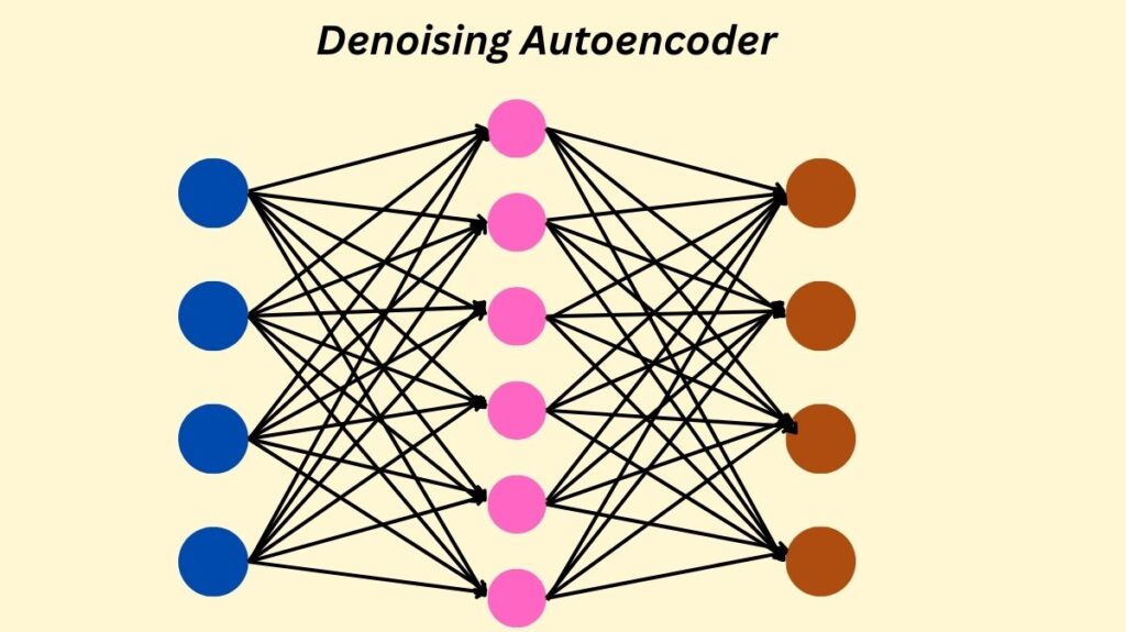
For unsupervised learning, one kind of neural network architecture is a denoising autoencoder (DAE). By learning to reconstruct the original, clean data from its noisy counterpart, it is essentially a variation of the original autoencoder that was created especially to eliminate noise from corrupted or noisy data. The main objective is to reduce the disparity between the reconstructed and original data. Through the prevention of overfitting, this ingenious method discourages the memorisation of minor information, improving the model’s ability to generalise to new data.

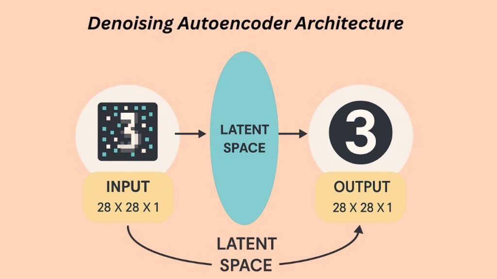
A DAE is supplied a noisy or corrupted version of the input to its encoder, as opposed to a typical autoencoder that receives the original input. Nevertheless, the loss of the decoder is only computed in relation to the original, uncorrupted input. This prevents the network from just replicating its input and forces it to learn how to reverse the damage. Because of this effective learning process, there is a much lower chance that the autoencoder will turn into an identity function, which would make the network unusable.

Humans frequently recognize targets even when an image is partially covered, and this human habit served as the impetus for the development of DAEs. High generalization ability is demonstrated by a DAE if it can rebuild clean data from noisy data.

Denoising Autoencoder Architecture

A Denoising Autoencoder is similar to a regular autoencoder in terms of architecture. There are two primary components to it:

Encoder:

• The neural network that serves as the encoder frequently has one or more hidden layers.
• Instead of receiving the original input, it gets the noisy data and creates an encoding in a lower-dimensional space. In other words, the encoder serves as a compression mechanism.
• Adding Gaussian noise or randomly masking portions of the inputs are the two most popular methods for creating corrupted input.

Decoder:

• A neural network with one or more hidden layers is used to implement the decoder, just as the encoder.
• It reconstructs the original data using the encoding that the encoder produced as input. A function of expansion is the decoder.
• Importantly, the loss function is computed by comparing the values of the reconstructed output with the original input rather than the corrupted input.

What DAEs Learn and How They’re Trained

By employing a corrupted input, the DAE is kept from turning into an identity function and the chance of overfitting is reduced. By forcing the network to prioritize the most important elements throughout the reconstruction process, it becomes noise-resistant.
A DAE’s training procedure usually consists of the following steps:

• Set random weights at the beginning for both the encoder and the decoder.
• To the initial clean input data, noise is purposefully introduced. This corruption can be accomplished using techniques such as:
  • Adding Gaussian noise.
  • A portion of the input is randomly set to zero in order to mask noise.
  • Salt-and-pepper noise, in which the maximum or minimum value of random pixels is set.
• To get the reconstructed output, the noisy input data is then passed through the encoder and decoder.
• The rebuilt output and the original, clean input are compared to determine the reconstruction loss.
• This reconstruction loss is minimized by updating the weights and doing backpropagation.
• Stochastic gradient descent (SGD) and its variations are examples of optimization algorithms that are commonly used for training.

Objective Function

Reducing the disparity between the original input (clean input free of noise) and the reconstructed output is the aim of a DAE. By employing a reconstruction loss function, this is measured. The type of input data determines which of two popular loss function types are used:

Mean Squared Error (MSE): Used for picture data input that contains floating pixel values, such as 0 to 255 or 0 to 1.

• MSE(x,y)=m1​Σi=1m​(xi​−yi​)2.
• In this case, x_i represents the input data’s pixel value, and y_i represents the reconstructed data’s pixel value, where y_i = D(E(x_i * \text{noise})) The decoder is denoted by D, and the encoder by E. The total of the training set is this.

Binary Cross-Entropy (log-loss): Used in cases where the input image data is made up of bit pixel values, meaning that the values are either 0 or 1.

• LL(x,y)=−m1​Σi=1m​(xi​ln(yi​)+(1−xi​)ln(1−yi​)).
• y_i is the pixel value of the reconstructed data, where y_i = D(E(x_i * \text{noise}), and x_i is the pixel value of the input data (0 or 1). The total of the training set is this.

Advantages and What DAEs Learn

Reconstruction error reduction improves feature extraction and generalization by teaching DAEs beneficial traits. They also offer a method for autoencoding high-capacity, overcomplete models without letting them learn the identity function.

Robust Feature Extraction: As they learn to extract robust features, DAEs that are trained with partially noisy inputs (such as Gaussian noise) have a tendency to generalize effectively to unseen, real-world data with varying degrees of noise or corruption. Applications where data quality is affected, such signal processing or image denoising, benefit from this. When it comes to learning features, DAEs outperform regular autoencoders.

Handling Incomplete Data: During the reconstruction process, DAEs learn to impute or fill in missing information if they are trained with partially damaged inputs (such as masking values). Because of this, they are helpful for jobs that require incomplete datasets.

Reduced Overfitting: In order to prevent overfitting and guarantee that the network learns meaningful representations, denoising the network prevents it from merely copying its input to the output.

Unsupervised Learning: The method does not require labelled data for training because it is unsupervised.

Applications of DAEs

DAEs’ capacity to handle noisy input and learn strong representations has led to their widespread use in a variety of applications.

Image Denoising: One of the most popular uses. DAEs are frequently used to eliminate noise from photographs, such as Gaussian or salt-and-pepper noise, in order to improve and clean them. They are able to extract a clear image from a noisy one.

Audio Denoising: DAEs are useful for speech-enhancement applications because they may be used to denoise audio signals.

Sensor Data Processing: They are helpful for processing sensor data, eliminating noise, and drawing out pertinent information from measurements.

Data Compression: DAEs and other autoencoders can be used to compress data by learning condensed representations of the input data.

Feature Learning/Extraction: Unsupervised feature learning works well with DAEs because they can identify pertinent features in the data without the need for explicit labels. This can help with classification and identification tasks.

Data Preprocessing: Before the data is used for training, they can successfully clean it up by preprocessing noisy data for other machine learning algorithms.

Anomaly Detection: After learning to recreate normal data, DAEs can detect anomalies in a dataset by identifying inputs that are hard to reconstruct (i.e., have a large reconstruction error) as perhaps abnormal. For instance, they can learn to rebuild normal transactions from noisy ones, which can be used to detect fraudulent transactions.

Data Imputation: DAEs can learn to rebuild the missing values from the remaining data in a dataset, allowing them to impute the missing values.

EEG Signal Classification: Low-dimensional representations of temporal and spectral inter-channel EEG connection matrices have been learnt by DAEs for classification tasks. It has also been suggested that stacked DAEs preserve local information in EEG dynamics to identify individualized characteristics in high-dimensional EEG indications.

Implementation Example (General Steps)

Examples of DAE implementations utilizing PyTorch and Keras; these are usually for image denoising tasks using datasets such as MNIST. The general procedures consist of:

Import Libraries: Numpy, matplotlib, torch (or tensorflow.keras), and torchvision (or tensorflow.keras.datasets) are imported as necessary libraries.

Define Dataloader/Load and Preprocess Data:

• Open the dataset (such as MNIST).
• Normalize pixel values (e.g., to 0-1 range).
• Add noise to the input data to create the corrupted versions. This is done by adding a random component (e.g., torch.randn for Gaussian noise or np.random.normal in NumPy) to the original clean data. The noisy data is then clipped to ensure it remains within valid pixel ranges.

Define the Model:

• Create a neural network class (e.g., DAE in PyTorch) that inherits from nn.Module or use the Keras functional API.
• Define the encoder (e.g., fc1, fc2, fc3 layers in PyTorch or Conv2D, MaxPooling2D layers in Keras) and decoder (e.g., fc4, fc5, fc6 layers in PyTorch or Conv2D, UpSampling2D layers in Keras).
• Use appropriate activation functions (e.g., ReLU for hidden layers, Sigmoid for output layer to squash values between 0 and 1).
• The forward method (in PyTorch) or the model definition in Keras will define how the noisy input is passed through the encoder and then the encoded representation through the decoder.

Define Optimizer and Loss Function:

• Choose an optimizer (e.g., Adam or SGD) to update model parameters during training.
• Select a loss function (criterion), typically Mean Squared Error (MSE) for float pixel values or Binary Cross-Entropy for binary pixel values.

Train the Model:

• Loop for a specified number of epochs.
• For each batch of data:
  • Clear gradients.
  • Add noise to the current batch of data.
  • Pass the noisy data through the model to get the reconstructed output.
  • Calculate the loss between the reconstructed output and the original, clean data.
  • Perform backpropagation and update weights using the optimizer.
• Monitor training progress by printing loss periodically.

Evaluate Performance/Denoise Images:

• Use the trained model to make predictions on noisy test data.
• Visualize the results by displaying the original, noisy, and reconstructed (denoised) images side-by-side to visually assess the model’s ability to remove noise and reconstruct the original.

Limitations

While DAEs are powerful, they do have some limitations:

• The choice and level of noise can significantly affect the model’s performance and may require careful tuning.
• Like other neural networks, DAEs can be computationally intensive to train, especially for large datasets or complex architectures.
• Although they are designed to remove noise, if not properly regularized, they may still lose some detail or relevant information in the data. For example, images might appear slightly blurry after denoising.
• The process of artificially adding noise before each training step increases the amount of calculation and processing time.
• Adding too much noise can lead to severe distortion of the input samples, potentially reducing the algorithm’s performance