Extreme Learning Machines (ELMs), a notable advancement in artificial neural networks, are renowned for their powerful performance on a wide range of tasks and their quick learning speed.
Introduction

One training approach for single hidden layer feedforward neural networks (SLFNs) is called Extreme Learning Machine (ELM). ELM sets itself apart with its distinct single-step training methodology, in contrast to conventional neural networks that employ iterative training techniques like backpropagation. Both supervised and unsupervised learning issues can be solved with it as a machine learning system. ELM has become well-known for its remarkable generalization performance, lightning-fast learning speed, and simplicity of use. It is frequently used for regression, grouping, and classification in real-time learning problems.
History of Extreme Learning Machine
Guang-Bin Huang et al. introduced the idea of ELM in 2006. However, the fundamental concept of randomizing some weights to lower learning difficulty was not wholly novel; it has previously been investigated in convolutional learning (1989) and reservoir computing (2002). ELM is a specific type of RVFL, or Radial Basis Function Neural Network (RBFNN), which uses random hidden weights and biases. The Schmidt Neural Network (SNN) and Random Vector Functional Link Net (RVFL) also predate ELM by more than ten years.
A unified learning framework for generalized SLFNs was the focus of ELM research from 2001 to 2010, which effectively demonstrated its universal approximation and classification capabilities. Research on kernel learning and common feature learning techniques like Principal Component Analysis (PCA) and Non-negative Matrix Factorization (NMF) expanded between 2010 and 2015. This research suggested that ELM might provide better or comparable results to SVM and could include PCA and NMF as special cases.
In addition to biological research bolstering some ELM theories, there was a greater emphasis on hierarchical ELM implementations between 2015 and 2017. Low-convergence problems have been addressed since 2017 by regularisation and decomposition techniques such as LU decomposition, Hessenberg decomposition, and QR decomposition.
Architecture of ELM
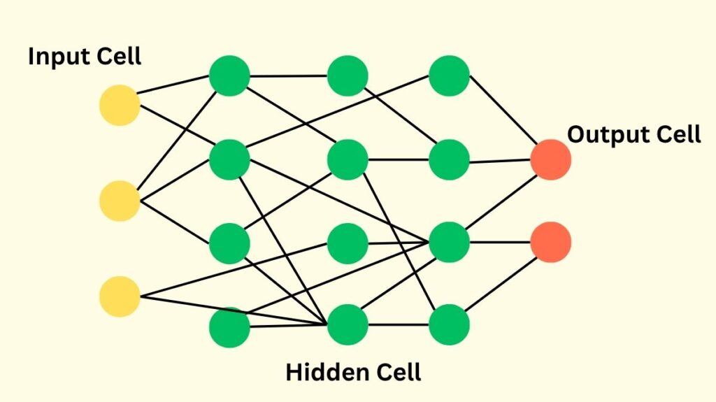
ELM has a clear and uncomplicated architecture with three main layers:
Input Layer: The raw data, expressed as an input vector with input features or attributes, is transferred to this layer.
Hidden Layer (Single Hidden Layer): In ELM, the biases in the hidden layer and the weights that link the input features to the hidden neurons are initially initialized at random and then frozen during the training procedure. The hidden layer gives the system nonlinearity by converting the input data into a high-dimensional feature space using nonlinear activation functions (such as sigmoid, hyperbolic, hardlimit, Gaussian, multiquadrics, or wavelet functions). One hyperparameter that must be established prior to training is the number of hidden neurons.
Output Layer: The only parameters that require learning are the output weights, also referred to as beta (β), which are the weights between the output layer and the hidden layer.
Also Read About Kohonen Networks and its Structure and Architecture
How Extreme Learning Machine Works
There are two primary steps in ELM’s basic training:
Initialization at Random
- The biases in the hidden layer (b) and the weights between the input and hidden layer (w) are assigned at random.
- Throughout the training process, these randomly chosen parameters are frozen and never changed.
- These random settings and nonlinear activation functions are used to map the input data into a random feature space. This mapping of random features adds to ELM’s capacity for universal approximation.
Linear Parameter Resolution
- An output matrix (H) is produced for the hidden layer following the processing of the input data using the fixed random weights and biases.
- Then, in a single step, the output weights (β) that link the hidden layer to the output layer are computed analytically.
- The usual method for performing this computation is to use the Moore-Penrose generalised inverse of the hidden layer output matrix (H) to solve a linear problem. Even for non-square or singular matrices, the Moore-Penrose inverse approximates the solution to linear equations by minimising squared errors or offering solutions with the minimum norm.
- ELM converges far more quickly than conventional gradient-based algorithms like backpropagation because of its non-iterative learning process.
Uses of Extreme Learning Machines
Real-Time Signal Processing
- Speech Recognition and Real-Time Signal Processing
- Classification of biological signals and EEG
- Monitoring of industrial sensors
Computer Vision
- Classifying images using computer vision (e.g., handwritten digit recognition)
- Detecting objects (in conjunction with feature extractors)
- Analysis of facial expressions
Predicting stock prices through financial forecasting
- Fraud detection
- Strategies for trading using algorithms
Automation in Industry
- Identifying defects in machinery
- Predictive upkeep
- Control systems for robotics
Natural Language Processing (NLP)
- Text classification using natural language processing (NLP) (e.g., spam detection)
- Analysis of sentiment
- Extraction of keywords
Features/Capabilities of ELM
Extreme Learning Machine provides a number of essential features and functionalities that enhance its efficacy:
Quick Training Speed
Because Extreme Learning Machine learns without iteration, it converges far more quickly than conventional gradient-based algorithms.
Good Generalization Performance
Despite having little training data, ELM typically produces promising results and a great capacity for generalization, which reduces its susceptibility to overfitting.
Universal Approximation Capability
Extreme Learning Machine has the capacity to estimate any continuous target function by using random hidden nodes and nonconstant piecewise continuous activation functions.
Classification Capability
ELM has good classification performance by successfully separating arbitrary disconnected sections of any shape.
Robustness
By using the Moore-Penrose generalised inverse to determine output weights, ELM is able to handle noisy and incomplete training data with ease. Additionally, it is resilient to user-specified variables.
Easy Implementation
With open-source libraries available, ELM is thought to be reasonably easy to implement.
Flexible Activation Functions
Sigmoid, Fourier, hardlimit, Gaussian, multiquadric, and wavelet functions for the real domain, and circular or hyperbolic functions for the complex domain, are just a few examples of the diverse array of nonconstant piecewise continuous functions that can be employed as activation functions in ELM’s hidden neurones.
Unified Learning Platform
ELM offers a unified learning platform for diverse neural network types, such as fuzzy inference systems, RBF networks, threshold networks, SLFNs, and more.
Also Read About What is an LSTM Neural Network and, Applications of LSTM
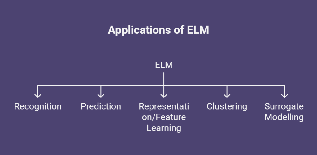
Applications of ELM

ELM is widely used in many different domains and machine learning tasks due to its exceptional training speed, accuracy, and generalization:
Recognition
Applied to the identification of objects, handwritten characters, aircraft, fabric defects, hyperspectral images, intrusion detection, bearing faults, palm prints, human facial expressions, and sensor-based activities.
Prediction
Used in a variety of prediction problems, such as predicting the pressure in coal slurry pipelines, predicting the melt index in propylene polymerization, predicting short-term loads, predicting bankruptcy, predicting greenhouse temperature and humidity, predicting solar radiation, predicting the price of carbon, predicting disease counts, predicting electric load and price, and predicting passenger flow. Forecasting economic growth is another use for it, and it is frequently based on data from the industry, trade, energy use (CO2 emissions), and research and technology advancement.
Representation/Feature Learning
The process of learning and extracting features from data is called representation/feature learning. This involves creating multilayer networks from ELM-AE for hierarchical representation, integrating deep belief networks with ELM for feature mapping, and employing ELM-AE for unsupervised feature learning and sparse representation.
Clustering
This method groups data and looks for patterns to solve unsupervised learning issues.
Surrogate Modelling
Used as a surrogate model or meta-model in optimization problems including soil slope reliability analysis, bottleneck stage scheduling, and multi-objective optimization.
Additionally, ELM is frequently used in a number of specialized fields:
Medical Application: Widely used in RNA classification, EEG analysis for epileptic seizure detection, and medical imaging (MRI for brain analysis, CT for liver/lung disease diagnosis, ultrasound for thyroid nodules, and mammogram for breast cancer detection).
Chemistry Application: Used to predict nonlinear optical properties, protein-protein interactions, toxicity of ionic liquids, Henry’s law constant of CO2, variables in chemical processes, and green management in power generation.
Transportation Application: Used for real-time driver attention detection, road surface temperature forecast, railway networks’ dynamic delay prediction, traffic sign recognition, traffic accident analysis, and taxi driver route recommendations.
Robotics Application: Used for robotic motion control, robotic arm control, object grasping detection, and electroencephalogram (EEG) signal classification in brain-computer interfaces.
IoT Application: Used in IoT contexts for intrusion detection, bug-fixing task assignment, and cyberattack detection.
Geography Application: Used to map the vulnerability of landslides, assess the stability of breakwaters on rubble mounds, forecast the carrying capacity of sediments, and determine the operating guidelines for hydropower reservoirs.
Food Industry Application: A widely used instrument for food safety, such as food safety monitoring systems, wine classification, large-scale food sampling analysis, predicting dairy food safety, categorising wheat kernels, and identifying the nitrogen concentration of amino acids in soy sauce.
Additional Multidisciplinary Uses: These include video analysis (e.g., moving cast shadow identification, video watermarking, violent scene detection), and control systems (e.g., adaptive control, automotive engine idle speed management).
