What is Real Time Recurrent Learning?

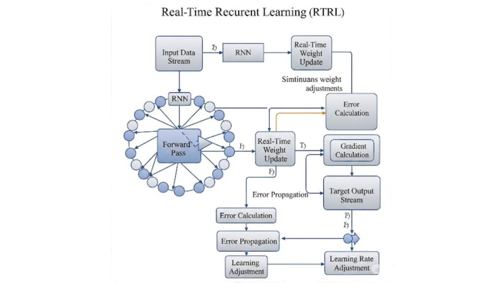
A learning technique called Real-Time Recurrent Learning (RTRL) was created for recurrent neural networks (RNNs) that process sequences. Backpropagation Through Time (BPTT) and other popular learning algorithms are conceptually different from it. With its emphasis on enabling online learning, RTRL is especially well-suited for control problems and real-time applications where prompt adaptation is essential. This means that the model may learn and change its parameters as new data becomes available.
The design of controllers for Multi-Input Multi-Output (MIMO) systems, such an autonomous helicopter model, can make use of RTRL in the context of control systems.
History of Real-Time Recurrent Learning
Although numerous authors separately developed RTRL, Williams and Zipser (1989b) are the most frequently acknowledged source. Many recommendations have been made to increase its learning speed and convergence since it was first introduced in 1989. Research has examined its potential applications in a number of contexts throughout the years, including when combined with policy gradients for actor-critic techniques.
How Real-Time Recurrent Learning(RTRL) Works?

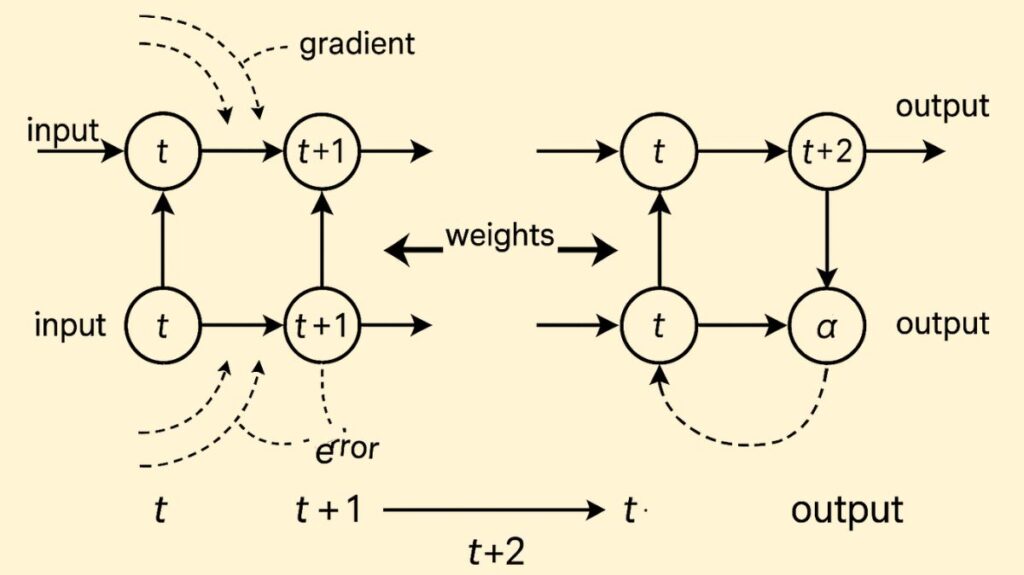
The idea behind RTRL is that gradient information is propagated forward in time. As the network analyses a sequence, RTRL computes the derivatives of states and outputs with respect to all weights, in contrast to classical backpropagation, which computes gradients by propagating mistakes backward. This implies that the gradient for the subsequent time step (t+2) is calculated using the gradient information from the previous time step (t+1), and so on.
Measuring the sensitivity of a unit’s output at a specific moment to a slight alteration in any network weight while taking into account the impact of that weight change across the network’s trajectory up to this point is the main principle. At every time step, this sensitivity data is gathered. Some of the terms in the gradient computation disappear because inputs usually don’t depend on network parameters. At each time step, the method recursively calculates these sensitivities, beginning with an initial condition that assumes the starting state is independent of the weights.
Two Real-Time Recurrent Networks (RTRNs) with the same network architecture are frequently utilized in learning control systems:
- The non-linear system is approximated by one RTRN.
- The other RTRN imitates the output of the intended system response.
These two RTRNs are combined to create the neural network control system, which implements the learning rule. They are trained using an iterative learning control (ILC) algorithm, in which weights learnt in one time step are applied in the subsequent one. Each RTRN variable is reliant on two independent variables throughout the learning process: time and iteration. Both RTRNs are trained consecutively until the error falls below a predetermined threshold. A control rule that changes control inputs to approximate the system output to the desired output is then created using the learnt weights.
Also Read About Convolutional Neural Networks Architecture and Advantages of CNNs
Advantages of Real-Time Recurrent Learning
RTRL is conceptually superior than Backpropagation Through Time (BPTT) in a number of ways.
- Online Learning: Since RTRL is an online or real-time technique, it may update model parameters following each pair of inputs and outputs. For many control problems, the model learns as data comes in, eliminating the requirement to gather data over time and then utilise it to train the model.
- No Caching Past Activations: Caching past activations is not necessary for RTRL.
- No Context Truncation: It can learn arbitrary long-term dependencies without truncation bias because it does not require truncating context.
- Programming and Derivation Ease: RTRL is simple to design and implement for novel network topologies.
- Unbiased Gradients: The ability to compute unbiased gradients is crucial for theoretical convergence guarantees in RTRL-based methods, particularly enhanced variants such as KF-RTRL.
Disadvantages and Limitations of RTRL
Despite its benefits, RTRL has serious flaws that prevent it from being used in big networks in its original configuration:
- High Time Complexity: The time complexity of the original RTRL method is O(n^4), where ‘n’ is the number of processing units in a recurrent network that is completely connected. Because of this, it is quite computationally costly and slow for big networks.
- High Space Complexity: It is unsuitable for large-scale applications due to its O(n^3) memory storage requirements.
- Multi-Layer Complexity: One constraint that is rarely addressed in practical applications is its complexity in the multi-layer case.
- Sensitivity to Initial Values: The model may occasionally exhibit non-convergence due to its sensitivity to weight initialisations.
- Noise in Approximations: While some approximations, such as UORO, introduce noisy gradients, others, like others, address complexity and can slow down learning.
Important RTRL Features and Characteristics
- Gradient-Based Learning: The RTRL algorithm propagates derivatives forward in time using gradients.
- Online/Real-Time Operation: This method is essentially an online learning approach that works well with real-time adaption and continuous data streams.
- Non-Local Effect Consideration: Even if the weight is not directly connected to the output unit, RTRL takes into account the impact of the change throughout the network trajectory when determining how sensitive an output is to a weight change.
- Adaptability in Control Systems: where network weights are dynamically changed throughout the control process, it can be viewed as a subsystem of an adaptive control system.
- Iterative Training: To reduce error, weights are adjusted over time steps and iterations in an iterative learning control (ILC) approach, which can be used to train RTRNs.
Also Read About Kohonen Networks and its Structure and Architecture
Types and Improvements of RTRL
The majority of subsequent work focusses on approximation theories to get around the original RTRL’s impracticality. To enhance RTRL, several strategies have been developed, which are frequently divided into gradient-based and stochastic-based approaches:
Cellular Genetic Algorithms, Mode Exchange RTRL (MERTRL), and sub-grouping strategies were investigated as means of enhancing learning speed and convergence. Among gradient-based algorithms, the original RTRL had the lowest error but the longest training time, while the sub-grouping technique was determined to have the worst convergence. When gradient-based techniques don’t work, cellular genetic algorithms have been found to be a viable substitute.
Element-wise Recurrence Neural designs: By concentrating on particular neural designs with element-wise recurrence, it is possible to achieve tractable RTRL without approximation, which permits scaling to difficult tasks such as DMLab memory tasks.
Decomposition/Learning in Stages: Breaking the network up into separate modules or learning the network in stages are two suggested limitations to make RTRL scalable. Without introducing bias or noise into the gradient estimate, these techniques seek to scale linearly with the number of parameters.
Online Recurrent Optimisation Without Prejudice (UORO)
The UORO algorithm reduces the runtime and memory cost of gradient approximations to O(n^2), which is comparable to a single forward pass in an RNN, hence mitigating the high computational requirements of RTRL. Convergence requires an objective estimation of the gradients, which UORO offers. But the drawback of this approximation is that it produces noisy gradients, which can slow down learning. It uses the outer product of two vectors to approximate the gradient of the hidden state with respect to parameters. Any RNN architecture can be used with UORO.
RTRL Factored by Kronecker (KF-RTRL)
- Another online learning technique that enhances UORO is KF-RTRL. It uses a Kronecker product decomposition to estimate the gradients.
- Unbiased Estimate: The gradients are estimated objectively by KF-RTRL.
- Less Noise: One major benefit is that KF-RTRL introduces noise that is consistent over time and substantially less (asymptotically by a factor of “n”) than UORO. Learning is significantly enhanced by this decreased variation.
- Cost of computation: KF-RTRL needs O(n^2) memory and O(n^3) operations. Its smaller variance frequently results in greater performance, even if its runtime is longer than UORO (O(n^2)).
- Applicability: KF-RTRL may be extended to LSTMs and is applicable to a broad class of RNNs, including popular architectures like Tanh-RNN and Recurrent Highway Networks.
- Empirical Performance: On real-world tasks such as character-level language modelling on the Penn TreeBank dataset, KF-RTRL has been demonstrated to nearly match Truncated BPTT’s performance. It also successfully captures long-term dependencies in tasks such as binary string memorisation.
Also Read About Gated Recurrent Unit (GRU) And its Comparison with LSTM
Applications of RTRL
RTRL and its enhanced versions have been used and evaluated in a number of fields:
Reinforcement Learning (RL) Tasks
ProcGen, Atari-2600, and DMLab-30 subsets have been used to test RTRL, which has been investigated in actor-critic techniques in conjunction with policy gradients. When compared to baselines such as IMPALA and R2D2, systems that use RTRL have demonstrated competitive or better performance in DMLab memory tasks while utilising a much smaller number of environmental frames.
Control Systems
It is used to approximate and control unknown nonlinear systems through online learning in the design of controllers for Multi-Input Multi-Output (MIMO) systems, as illustrated using an autonomous helicopter model.
Modelling and Prediction
RTRL has been used to solve temporal process-related challenges including:
- Resolving chronic dependency issues.
- Simulating the classical deterministic chaos model, the Hénon map.
- Forecasting an NH3 laser’s chaotic intensity pulsations.
Converting text to phonemes
A quick RTRL algorithm has been used for this purpose.
Character-Level Language Modelling
The Penn TreeBank dataset has been used to assess KF-RTRL for character-level language modelling, a difficult task that calls for both short-term and long-term dependencies.
Also Read About What are the Radial Basis Function Networks?
Comparison with Backpropagation Through Time (BPTT)
Two well-known gradient-based techniques for recurrent learning with unique features are RTRL and BPTT:
Online vs. Offline Learning
After every input/output pair, the parameters of the online learning algorithm RTRL are updated. The complete sequence (or a reduced portion) must be processed before calculating gradients and updating parameters in BPTT, which is often an offline technique.
Memory and Time
Although BPTT particularly Truncated BPTT, or TBPTT is frequently employed in practice, if the truncation horizon is too tiny, it is limited in its capacity to acquire very long-term dependencies due to truncation bias. Long sequences take a lot of memory because it also has to store previous states. By avoiding context truncation and the necessity to cache previous activations, RTRL seeks to get around these restrictions. However, compared to TBPTT (which has an O(n^2) runtime when truncated), the original RTRL was historically unworkable due to its high time (O(n^4)) and memory (O(n^3)) complexity.
Gradient Propagation
Gradients are propagated forward in time by RTRL and backward in time by BPTT.
Equivalence for Batch/Pattern Updates
Because they compute the identical derivatives, RTRL and BPTT are comparable for batch and pattern weight updates.
Additional Insights and Experimental Findings
Tractability
Research frequently concentrates on neural architectures with element-wise recurrence, which enable tractable RTRL without approximation, in order to scale RTRL to difficult challenges.
Convergence
Although RTRL (and its precise gradient computation) can attain minimal error, it frequently necessitates a longer training period in contrast to certain quicker but less precise techniques.
Approximation Variance
The rate of convergence is closely correlated with the variance of gradient estimates. Learning is slowed down by algorithms like UORO, which introduce a lot of variance. KF-RTRL is a more successful online learning strategy since it targets and significantly eliminates this noise.
Online Updates and Learning Rate
In practice, RTRL’s online updates only make the estimated gradient accurate up to a certain point, which is typically not a problem at small enough learning rates.
Enhancing Online Learning Algorithms
By resetting gradient approximations and eliminating “stale gradients,” methods such as resetting the hidden state with a tiny probability (as employed in Penn TreeBank studies) can aid online learning algorithms.
