Boltzmann Machine Neural Networks
One kind of neural network that may make stochastic judgements is a Boltzmann Machine (BM), which is made up of linked neurons. Geoffrey Hinton and Terry Sejnowski created it in 1985. BMs, which are regarded as unsupervised deep learning models, are distinguished by their symmetrically linked units and recurrent structure.
Purpose and Objective
Search problems and learning issues were the two primary computing difficulties that Boltzmann machines were first designed to solve.
- The weights on connections, which reflect the cost function of an optimization issue, are fixed for search tasks. The BM may then sample binary state vectors that reflect excellent solutions with its stochastic dynamics.
- A dataset of binary vectors is given to the BM for learning problems, and it must assign weights to its connections in order for the data vectors to be effective solutions to the optimization problem that those weights specify.
A Boltzmann machine’s main goal is to optimize a problem’s solution by modifying its weights and quantities. Using samples, they seek to understand the key components of an unknown probability distribution as well as the internal representations of input. Through unsupervised learning techniques like clustering, dimensionality reduction, anomaly detection, and generative models, BMs are also used to generate mappings and learn from characteristics and target variables, especially for locating underlying structures or patterns in data.
Boltzmann Machines Architecture

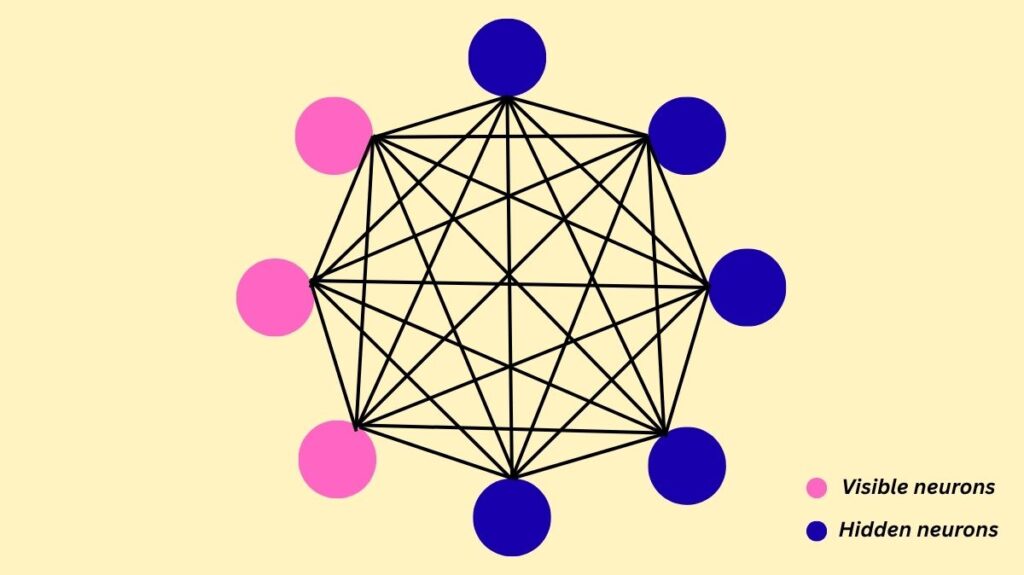
A collection of symmetrically linked neurons that make stochastic decisions such as whether to be on or off, or 1 or 0 make up a Boltzmann machine. There are two primary categories of nodes or units in it:
Visible neurons/nodes: These are the nodes that are observable or measurable.
Hidden neurons/nodes: These nodes are either not described by the observed data or cannot be measured. By acting as latent variables or features, they allow the BM to represent intricate distributions across observable state vectors, something that is not possible with just direct pairwise interactions.
One important feature of a Boltzmann Machine is that, in contrast to many other neural networks, all nodes whether input (visible) or hidden are linked to all other nodes. A completely linked graph is produced as a result. Bidirectional connections exist between units, therefore wij = wji. Self-connections (wii) are another possibility.
How Boltzmann Machines Work

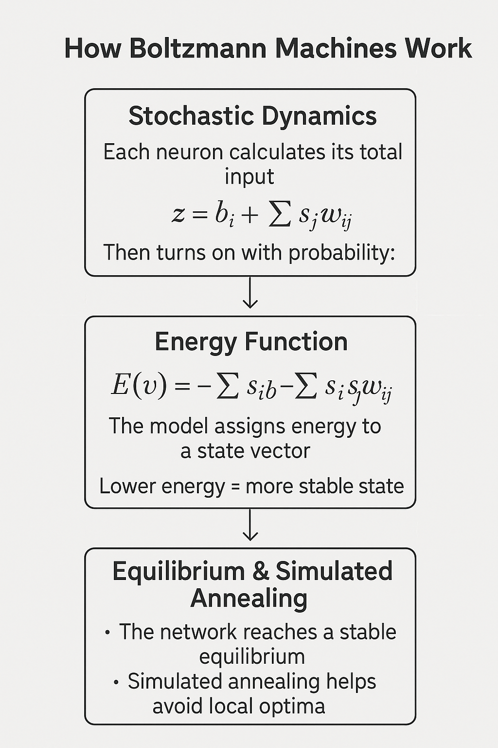
Instead of being deterministic, Boltzmann Machines are generative or stochastic Deep Learning models. Their goal is to reduce the model’s “energy” by making minor adjustments to their weights.
Stochastic Dynamics: A unit (neuron i) initially determines its total input (zi) before updating its binary state (0 or 1): Zi = bi + ∑j sjwij In this case, sj is the state of unit j (1 if on, 0 otherwise), wij is the weight on the connection between unit i and unit j, and bi is the bias of the unit. The logistic function then determines the likelihood at which unit I turns on: 1 / (1 + e−zi) = prob(si = 1)
Energy Function: The energy function E(v), where v is a state vector that represents the binary states of all units, defines the behavior of a Boltzmann machine. The energy determines the “badness of state,” therefore stability is indicated by a minimal energy and a lower energy is beneficial for the model. The standard definition of the energy function is E(v) = −∑i sibi − ∑i<j sisjwij. In this case, wij is the weight between units I and J, si is the binary state of unit I, and bi is the bias. According to the Boltzmann distribution, the energy of a state vector v in relation to all other potential binary state vectors determines its probability: e−E(v) / ∑u e−E(u) = P(v)
Equilibrium and Simulated Annealing: The network will ultimately achieve a stable or equilibrium state, sometimes referred to as a Boltzmann distribution, if units are updated successively. Because of the stochastic dynamics, the BM can hop over energy barriers and escape from bad local optima by periodically raising its energy during the search. Simulated annealing, which entails progressively lowering a “temperature” parameter (T) to gain from quick equilibration at high temperatures and reach a final equilibrium distribution where excellent solutions are more likely, might improve this search procedure. A Boltzmann machine turns into a Hopfield network at zero temperature.
Learning in Boltzmann Machines
Finding the weights and biases that create a Boltzmann distribution with a high probability for the training vectors is the process of learning in a Boltzmann machine. Gradient ascent in the log likelihood that the BM would produce the observed data is used to do this. The difference between two correlations provides the learning rule for weights (wij): δ(log P(v))/δwij = data − \sisj>model
<sisj>data: When a data vector is clamped on the visible units and the hidden units are updated until they achieve equilibrium, the predicted value of sisj is obtained. This is sometimes referred to as the clamped phase or the positive phase. It is an example of Hebbian learning, in which neurons are strengthened by their simultaneous firing.
<sisj>model: The anticipated value when state vectors from the equilibrium distribution are freely sampled by the Boltzmann Machine. This can be viewed as a “forgetting” or “unlearning” contribution and is also referred to as the negative phase or free-running phase.
Since the time needed to train the model grows exponentially with size, learning in unconstrained Boltzmann machines is sluggish and impracticable owing to their completely linked nature. Converging to local minima is another issue they deal with.
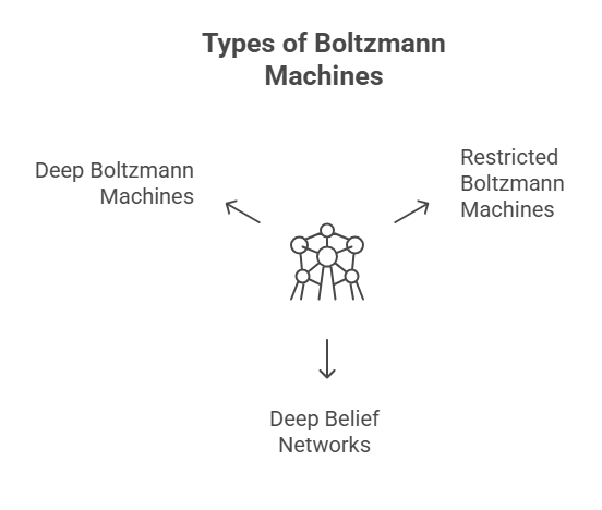
Types of Boltzmann Machines
Variants with limited connections were created in order to get around the original Boltzmann Machine’s drawbacks, especially its sluggish learning.

Restricted Boltzmann Machines (RBMs)
Restriction: By prohibiting connections between nodes inside the same layer (i.e., no visible-visible or hidden-hidden connections), RBMs make the Boltzmann Machine simpler. As a result, the entire graph becomes bipartite.
Advantage: This limitation speeds up training and improves the model’s usefulness. Given a visible vector, hidden units are conditionally independent, enabling the acquisition of unbiased samples from the positive phase (data) in a single parallel step.
Training: RBMs use a technique known as Contrastive Divergence to modify their weights. This entails rebuilding the input following a few Gibbs sampling runs in order to approximate the model expectation. A quantity known as “contrastive divergence” is the result of this effective process’ approximate gradient descent.
Example (Recommender System): A recommender system may be constructed using an RBM. For example, an RBM learns to assign hidden nodes to certain attributes (e.g., “Drama” genre, “Action” genre, “Oscar” winner, “Dicaprio” actor) if a user like Mary watches and rates movies. Through an analysis of Mary’s preferences, the RBM determines which characteristics are significant to her. Then, if the attributes of unrated films match those of Mary’s favourite films (such as “Drama,” “Dicaprio,” or “Oscar”), it might suggest a film like “m6.”
Applications: Dimensionality reduction, collaborative filtering, topic modelling, classification, and feature learning are all common applications for RBMs. Because they can simulate continuous data present in natural pictures, they are very helpful in imaging and image processing.
Deep Belief Networks (DBNs)
Structure: Multiple RBMs are stacked on top of one another to construct probabilistic generative models known as DBNs. The visible layer of the subsequent RBM receives the output of the hidden layer of the previous RBM.
Connections: With the exception of the top two levels, which retain undirected connections to create an RBM, connections inside each RBM layer in a DBN are undirected, whereas connections between layers are often directed.
Training: Usually, DBNs are trained in two stages:
- Pre-training: Each RBM is trained hierarchically using a greedy layer-wise unsupervised pre-training technique, where weights and biases are established.
- Fine-tuning: The network as a whole is then adjusted using an up-down supervised learning technique. DBNs may also be trained using the Wake-Sleep Algorithm.
Applications: DBNs have been used for applications such as facial expression recognition, audio classification (voice activity detection), time-series forecasting, breast cancer classification, and hyperspectral spatial data classification because they are good at extracting features.
Deep Boltzmann Machines (DBMs)
Structure: Like DBNs, DBMs are generative models with units organized in layers.
Connections: The main distinction between DBMs and DBNs is that DBMs include undirected linkages across the whole structure, even between levels.
Learning: Similar to DBNs, DBMs learn by avoiding bad local minima and initializing weights through layer-by-layer pre-training. DBMs integrate top-down feedback, which aids with confusing inputs, and employ an approximation inference process with an extra bottom-up step to speed up learning.
Applications: DBMs are appropriate for jobs like voice and object identification since they are utilized to capture intricate underlying properties in data. They have been used in face modelling, 3D model recognition, spoken question detection, subject modelling, and multimodal learning.
Finally, Boltzmann Machines’ stochasticity and energy-based learning enabled complex generative models. Original BM’s fully connected structure and slow learning presented practical challenges, but RBMs, DBNs, and DBMs improved training algorithms and architectural constraints, making them widely used in deep learning tasks.
