A fundamental kind of artificial neural network that is essential to both machine learning and deep learning is the Multilayer Perceptron (MLP). Its layered structure and capacity to handle complicated data are its defining features. We described the Multilayer Perceptron in this article, including its definition, multilayer perceptron history, works, features, and backpropagation.
What is Multilayer Perceptron (MLP)?
A Multilayer Perceptron (MLP) is a kind of artificial neural network made up of several layers of hierarchically arranged neurons, sometimes referred to as perception elements or nodes. By employing many layers, MLPs get over the drawbacks of single-layer perceptrons, which are only useful for straightforward issues. This enables them to tackle more complicated problems and produce predictions that are more accurate.
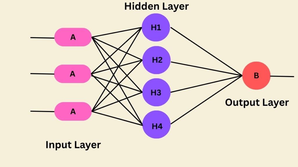
An MLP normally has a minimum of three structural layers:
- An input layer for data reception.
- Information processing through one or more hidden levels.
- The final forecast is provided by an output layer.
An MLP is called a deep artificial neural network (ANN) or deep neural network if it contains multiple hidden layers.
Feedforward artificial neural networks, of which MLPs are typical examples, transfer data from the input to the output in a single direction. They are frequently employed for problems involving supervised learning, such regression and classification.
Multilayer perceptron history

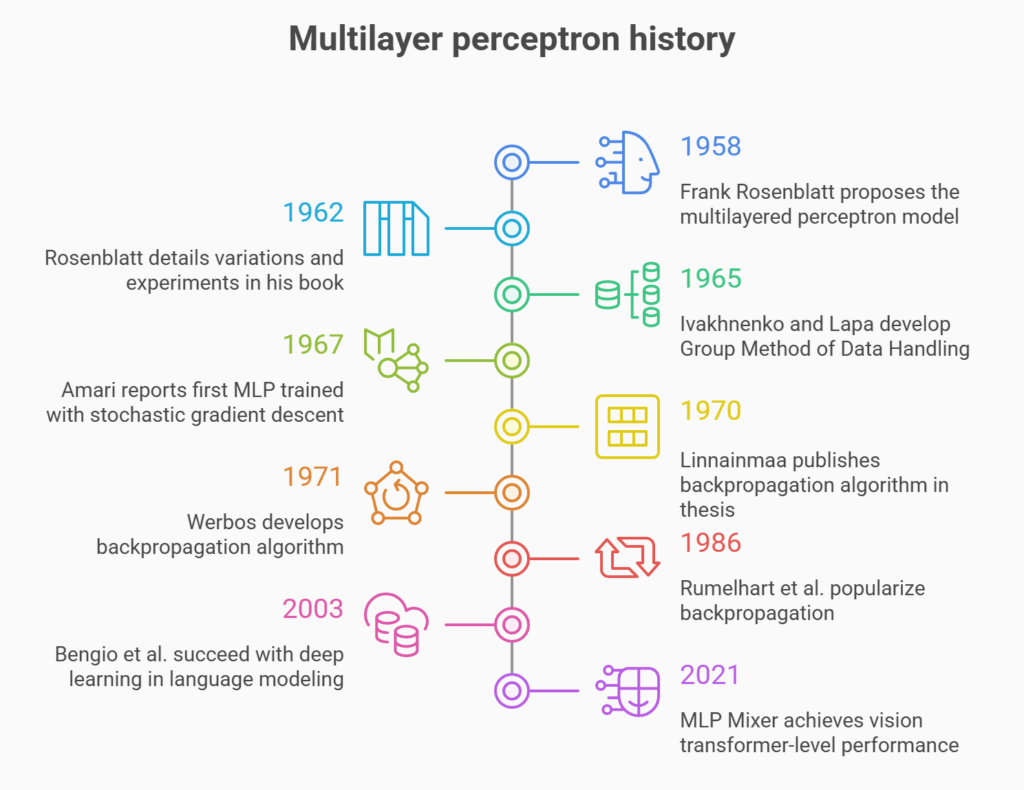
Following the invention of the Rosenblatt perceptron in the 1950s, interest in the idea of artificial neural networks began to wane. But when Dr. Hinton and his associates created the backpropagation technique for multilayer neural network training in 1986, interest was rekindled. With big businesses like Google, Facebook, and Microsoft making significant investments in their applications, deep neural networks which include MLPs are a very active field nowadays.
The multilayered perceptron model, which had an input layer, a hidden layer with randomised non-learning weights, and an output layer with learnable connections, was first proposed by Frank Rosenblatt in 1958. This is where the history of multilayer perceptrons (MLPs) begins. In his 1962 book Principles of Neurodynamics, Rosenblatt went into additional detail about variations and experiments that featured up to two trainable layers using a technique known as “back-propagating errors,” however this was not the generic backpropagation algorithm.
The limitations of single-layer perceptrons, which could only classify data that was linearly separable, were addressed with the development of MLPs. The 1965 Group Method of Data Handling by Alexey Grigorevich Ivakhnenko and Valentin Lapa, a deep learning technique that trained an eight-layer neural net by 1971, is another important early study on multi-layered neural networks.
The first multilayered neural network trained with stochastic gradient descent that could categorise non-linearly separable patterns was reported by Shun’ichi Amari in 1967. The backpropagation technique was independently invented by multiple people in the early 1970s; the oldest published example was Seppo Linnainmaa’s master’s thesis from 1970. This algorithm is essential for training contemporary MLPs with continuous activation functions. It was also developed in 1971 by Paul Werbos, who published it in 1982.
David E. Rumelhart et al. popularized this algorithm in 1986. Following Yoshua Bengio and co-authors’ success with deep learning in applications such as language modelling in 2003, interest in these networks began to grow again. In 2021, a novel architecture known as MLP Mixer which combines two deep MLPs showed picture classification performance on par with vision transformers.
How it Works

Data is processed by an MLP by moving it through a number of layers, each of which has a specific function:
- Input Layer: This is where raw data is introduced into the network. In this layer, each neuron usually reflects a feature of the input data.
- Hidden Layers: The majority of processing takes place in the hidden layers. They use mathematical processes to change the input data, frequently using non-linear activation functions as the Rectified Linear Unit (ReLU), hyperbolic tangent (tanh), or sigmoid. For the network to recognize complex patterns and resolve challenging issues like image processing, these non-linear functions are essential. Applying an activation function to a computed ‘z’ value yields an activation unit.
- Output Layer: This layer generates the network’s final output or prediction. It may produce probability for various categories in classification tasks and a single value in regression activities. Predicted class labels are often obtained by passing the output through a threshold function.
A Multilayer Perceptron modifies its internal parameters to reduce errors as it processes data by moving it through its layers in a predetermined order.
- Forward Propagation: From the input layer, data is sent to the output layer. Weights and biases are used by each layer to alter the data.
- Error Calculation: The error is determined by calculating the difference between the known actual outcome and the expected outcome based on the network’s output. It is necessary to minimize this error. This disparity is measured using a loss function (such as cross-entropy or mean squared error).
- Backpropagation: Beginning at the output layer and progressing to the input layer, the error is backpropagated throughout the network. The model’s weights and biases are adjusted to minimize the error by calculating the derivative of the error with respect to each weight in the network. This procedure, which is founded on the downward gradient approach, is also referred to as the generalized delta algorithm.
Also Read About What are the Radial Basis Function Networks?
Features of MLPs
MLPs have a number of essential characteristics that allow them to function:
- Fully Connected Layers: MLPs are referred to as completely connected layers since every node in one layer is connected to every node in the layer above and below it.
- Non-linear Activation Functions: They handle issues that are not linearly separable and model intricate, non-linear relationships in data by using non-linear activation functions in the hidden and output layers.
- Universal Approximators: Because MLPs can approximate any continuous function, they are referred to as universal approximators. They are therefore appropriate for nonlinear classification problems as well as nonlinear function approximation.
- Adjustable Parameters: The weights and biases of the network, which control the bias of each neuron and the strength of connections between neurons, can be changed to help the network learn.
- Hyperparameters: To maximize network performance, hyperparameters which include the number of layers and the number of neurons in each layer need to be carefully adjusted.
- Supervised Learning: Supervised learning methods, mainly backpropagation, are used to train MLPs. These methods require input-output data pairs.
Multilayer perceptron backpropagation
MLPs are trained using the backpropagation algorithm, a supervised learning method. Among its steps are:
- Initialisation: The perceptron’s weights are set at random (for example, between -0.1 and 0.1).
- Training Pattern Presentation: The perceptron is shown an input pattern from the training data.
- Forward Computation (Output and Hidden Layer): A sigmoid activation function is usually used to calculate the values of hidden-layer neurons. The values of the output neurons are then computed. The discrepancy between the intended and actual output is used to compute errors in the output layer. The output layer errors and weights are then used to compute the hidden-layer neuron errors.
- Backward Computation (Weight Adjustment): A learning rate (η) and the computed errors are used to modify the weights between the output layer and hidden layer. Weights between the input and hidden layers are also changed.
- Iteration: One cycle through the training set defines an iteration, and Steps 2–6 are repeated for every pattern vector in the training data.
Backpropagation training of an MLP can be slow; for large problems, it may take thousands or even tens of thousands of epochs. Learning can be accelerated by strategies like momentum and varied learning rates.
Also Read About What Is Single Layer Perceptron Neural network Architecture
