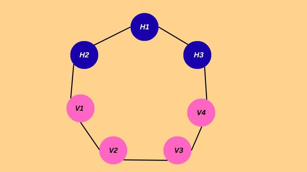
What is a Restricted Boltzmann machine?

One kind of Artificial Neural Network that functions as a probabilistic graphical model is called a Restricted Boltzmann Machines (RBM). This generative model can develop a probability distribution over a set of input data and is mainly used for Unsupervised Learning. Stochastic neural networks are the interpretation of RBMs.
RBMs were first presented by Hinton and Salakhutdinov in the middle of the 2000s. They are used to solve unsupervised learning issues and have drawn a lot of interest as components of multi-layer learning systems such as deep belief networks (DBN). In 1985, Geoffrey Hinton, who is frequently called the “Godfather of Deep Learning,” invented the Boltzmann Machine, of which RBMs are a particular type.
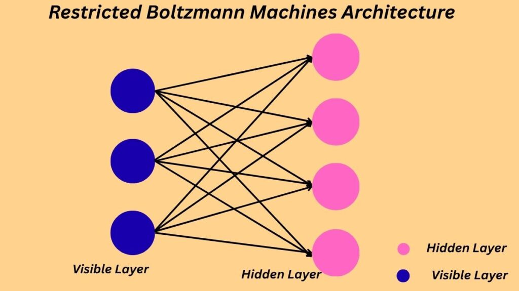
Restricted Boltzmann Machines Architecture

Two layers of neurons make up an RBM:
Visible Layer (or Input Layer): The input data is represented by this layer. The input features, which may be binary or real-valued, are represented by its nodes. In the visible layer, each neuron’s job is to look for patterns in the data.
Hidden Layer: This layer collects the underlying features or patterns in the data and reflects a collection of features that the network has learnt. The pattern seen by the visible neurons is explained by the neurons in the hidden layer. Generally speaking, there are fewer hidden nodes than visible ones.
A key architectural restriction is denoted by the term “restricted”: connections between neurons in the same layer are prohibited. Accordingly, only neurons in the hidden layer are connected to each neuron in the visible layer, and vice versa. An asymmetrical bipartite graph is created when every hidden node is connected to every visible node. The weights of the links between the layers are symmetrically connected.
Why the Restriction?
This limitation is crucial because it
- Streamlines the process of training.
- Improves learning efficiency and lowers computational complexity.
- Makes the RBM understand intricate linkages and dependencies between visible characteristics by forcing it to concentrate on their interactions.
- Simplifies probability calculations by establishing neuronal independence within a layer.
How Restricted Boltzmann Machines Work
In order to decrease the discrepancy between the input data and its reconstruction, RBMs learn the input data’s probability distribution through interactions between the visible and hidden layers. There are two primary stages to this iterative process:
Positive Phase (Feed Forward Pass / Reconstruction):
- A data point (activations of visible units) is fed into the RBM.
- The RBM activates hidden neurons based on weights and biases. The probability of a hidden node activating given the visible layer input v is calculated using a sigmoid function: P(hj=1∣v)=σ(bj+∑iviwij). \σ denotes the sigmoid function, b_j represents hidden node bias, v_i represents visible node state, and w_{ij} indicates weight between them.
- When there is a positive correlation between the visible and hidden units, this procedure finds positive relationships.
- Then, taking into account the hidden layer’s activity and the weights between it and the visible layer, the RBM recreates a new visible layer activation pattern. P(vi=1∣h)=σ(ai+∑jhjwij) yields the reconstructed visible v’i, where a_i is the bias of visible node i.
- A reconstruction of the initial input is then produced by sampling the visible states from this probability distribution.
Negative Phase (Feed Backward Pass / Learning):
- By feeding the network with the reconstructed visible layer activation, hidden neurons are activated using the reconstructed data.
- To identify differences, the RBM contrasts the buried layer’s activations from this phase with those from the first input (positive phase). This is where adverse correlations are found.
- The weights and biases are modified in light of this comparison in order to decrease the discrepancy between the reconstruction and the original data. Error = Reconstructed Input Layer – Actual Input Layer is how the error is computed.
- The gradient of the reconstruction error is frequently used to determine the weight adjustment; Contrastive Divergence (CD) is a popular technique. For instance, Δwij=ϵ(⟨vihj⟩data−⟨vihj⟩recon)Δai=ϵ(vi−vi′)Δbj=ϵ(hj−hj′) yields the weight update \Δ w_{ij}, where \ϵ is the learning rate.
- An RBM’s energy function is provided by E(v, h) = -a^T v – b^T h – v^T Wh. After training, the system adjusts the weights in an effort to determine the lowest energy state.
- Example: RBM can find latent factors (unobserved variables) that explain movie choices in a movie rating situation. If films like Avengers, Avatar, and Interstellar are frequently linked to “fantasy” and “science fiction,” for example, RBM can determine these underlying characteristics from user ratings. RBM is able to infer similar traits and make movie recommendations when a new user activates hidden units that are similar to those activated by a prior user.
Training of Restricted Boltzmann Machines
Contrastive Divergence (CD) is the main training method for RBMs. The stochastic gradient descent algorithm features a variation called CD. In order to decrease the reconstruction error, it iteratively updates the weights and biases to approximate the gradient of the log-likelihood function of the data. When it is difficult to evaluate probability or functions directly, this approach is employed.
Gibbs Sampling, a Markov Chain Monte Carlo (MCMC) approach used to approximate multivariate probability distributions, particularly when direct sampling is challenging, is another technique cited in relation to RBMs. MCMC techniques are the foundation of many RBM learning algorithms.
Types of Restricted Boltzmann Machines
According to the variables they employ, there are primarily two types:
Binary RBM: Binary variables, such as input and hidden units, are frequently used to model binary data, such as text or images.
Gaussian RBM: When modelling continuous data, such as audio signals or sensor data, input and hidden units are continuous variables with a Gaussian distribution.
Variations of RBMs include
Deep Belief Network (DBN): A generative model is made up of several layers of RBMs built one on top of the other, with each RBM’s output acting as its input. High-dimensional data, such as pictures or films, are frequently handled by DBNs.
Convolutional RBM (CRBM): With local and shared connections between units, it is intended for processing images or structures that resemble grids in order to record spatial relationships.
Temporal RBM (TRBM): With hidden units connected across time steps to depict temporal dependencies, it is intended for temporal data (such as time series and video frames).
Deep Boltzmann Machines (DBMs): Like DBNs, but able to extract more complicated features due to undirected connections both within and between layers.
Advantages and Disadvantages of Restricted Boltzmann Machines
Advantages
- Faster than typical Boltzmann machines because to the limited number of connections.
- Sufficiently expressive and computationally efficient to encode any distribution.
- Able to discover hidden patterns and connections in high-dimensional information and learn intricate probability distributions.
- Algorithms for unsupervised learning don’t need tagged input data.
- Other models can incorporate hidden layer activations as useful characteristics to improve performance.
- Useful for independent component analysis, feature extraction, and dimensionality reduction.
Disadvantages
- Computationally costly because they need a lot of iterations and the number of parameters grows exponentially, especially for huge datasets.
- When utilised as a single RBM, it has a limited potential to learn complex relationships.
- May have trouble training with incomplete or contaminated data.
- Setting up the right parameters (such learning rate) might be challenging and result in subpar performance.
- The intricacy of computing the energy gradient function makes training difficult.
- Backpropagation is more well-known than the CD-k method.
Applications of Restricted Boltzmann Machines
RBMs are widely used in many different domains, especially in deep learning and machine learning:
Collaborative Filtering and Recommender Systems: Widely used to propose interesting products and forecast user preferences based on historical behaviour. Amazon and Netflix are two examples.
Image and Video Processing: Utilized for tasks like as tracking, video segmentation, object recognition, picture denoising, and image reconstruction. For image identification, they can also pre-train layers in deep neural networks.
Natural Language Processing (NLP): Used in sentiment analysis, speech recognition, text categorization, language modelling, and speech synthesis.
Bioinformatics: Drug discovery, gene expression analysis, and protein structure prediction are a few examples of applications.
Financial Modelling: Utilized for projects like risk analysis, portfolio optimization, and stock price prediction.
Anomaly and Fraud Detection: Can be trained on big datasets to identify unusual or suspicious activity, including medical diagnosis, network infiltration, and financial transaction fraud.
Dimensionality Reduction: By efficiently reducing the amount of dimensions in data, RBMs are able to extract more significant characteristics and capture the most pertinent ones.
Feature Learning/Extraction: Features that are useful for other machine learning tasks can be learnt by RBMs from input data. For example, RBMs are employed to extract discriminative features before supplying them to a CNN for classification in handwritten digit recognition.
Classification and Regression: They are applied to a variety of regression and classification issues.
Topic Modelling: An example in which fewer unobserved variables are needed to characterise variability among correlated variables using RBMs.
Radar Intra-Pulse Real-Time Detection: Used to reduce noise and analyse the ambiguity function (AF) in radar signals in order to extract features. The processed data is then fed into a trained RBM for recognition.
Despite their strength, RBMs are not as frequently utilised alone these days; instead, deep feed-forward networks with multiple layers and regularisation strategies are more widely used. Nonetheless, they continue to make a substantial contribution to deep learning systems, especially as pre-training layers in DBNs.
Boltzmann Machines vs Restricted Boltzmann Machine
Artificial neural networks of the BM and RBM types are both used to learn Probabilistic Graphical Models. The main differences are:
Connections: Conventional Boltzmann machines have neurons that are intra-layer (connected to all other neurons), including those in the same layer. RBMs, on the other hand, only allow connections between the visible and hidden levels; intra-layer connections are strictly forbidden.
Complexity and Training: Because of this limitation, RBMs are a “special case” of Boltzmann Machines, which makes their implementation easier and enables them to train considerably more quickly than conventional BMs. RBMs are simpler to train and converge more quickly than BMs, despite BMs’ greater strength and ability to remember intricate distributions.
Output Layer: There is no explicit output layer in RBMs or Boltzmann machines.
Purpose: Both models learn probability distributions through generative unsupervised learning. Dimensionality reduction and the extraction of significant features are two areas in which RBMs excel.
