Practical Example of Linear Text Classification
Let’s look at a straightforward real-world example of using logistic regression to categorise movie reviews as either good or negative.
from sklearn.feature_extraction.text import CountVectorizer
from sklearn.linear_model import LogisticRegression
from sklearn.model_selection import train_test_split

# Example movie reviews
reviews = ["I love this movie", "This was a terrible movie",
"Absolutely fantastic!", "Not great, very boring"]

labels = [1, 0, 1, 0]  # 1 for positive, 0 for negative

# Convert text to Bag of Words
vectorizer = CountVectorizer()
X = vectorizer.fit_transform(reviews)

# Split into training and testing sets
X_train, X_test, y_train, y_test = train_test_split(X, labels, test_size=0.25)

# Train a Logistic Regression classifier
model = LogisticRegression()
model.fit(X_train, y_train)

# Make predictions
predictions = model.predict(X_test)
print(predictions)
In this straightforward example, a few movie reviews are converted into a numerical format using Bag of Words, and then they are classified as favourable or negative using logistic regression.
Although Bag of terms is a straightforward and popular approach, there are other, more sophisticated methods for representing text in Natural Language Processing. One of these is TF-IDF (Term Frequency-Inverse Document Frequency), which is a variation of BoW that prioritises uncommon terms over common ones.
What is TF-IDF?
Natural Language Processing uses the TF-IDF, a numerical statistic, to assess a word’s importance in a document relative to a corpus, or group of documents. By emphasising terms that are common in a particular document but less common in many others, TF-IDF aims to make those words more significant or unique to that document.
Components of TF-IDF
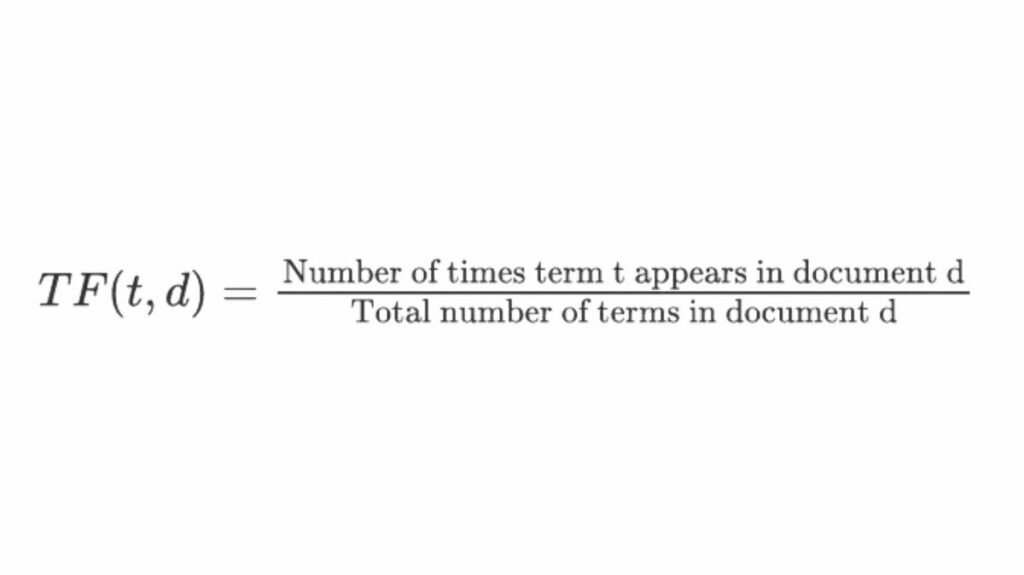
A term’s term frequency (TF) indicates how often it occurs in a document. It is the document’s word count in its raw form.

By using Inverse Document Frequency (IDF), terms that occur often in several documents are given less weight. A word is deemed less informative if it appears frequently in papers.

TF-IDF Rating
The TF and IDF values of a word in a document are multiplied to determine its final TF-IDF score:

Higher TF-IDF scores will be assigned to words that appear frequently in one document but infrequently in many others.
Example of TF-IDF Calculatio
Assume you have three texts in your corpus:
- “I adore machine learning.”
- “Deep learning is something I adore.”
- “Deep Blue is an automated chess player.”
Objective
The TF-IDF score for the word “machine” in the first document is what it wish to determine.
Methodical Calculation
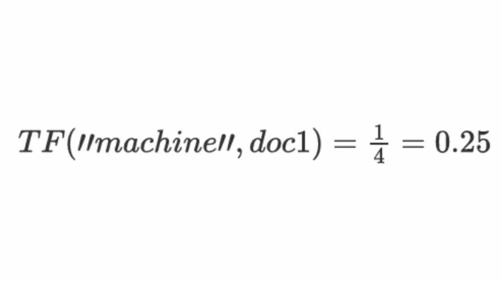
Step 1: Calculate Term Frequency (TF)
The term “machine” appears once out of four words in the first document. Thus:

Step 2: Calculate Inverse Document Frequency (IDF)
Two of the three documents (documents 1 and 3) contain the word “machine.” Thus:

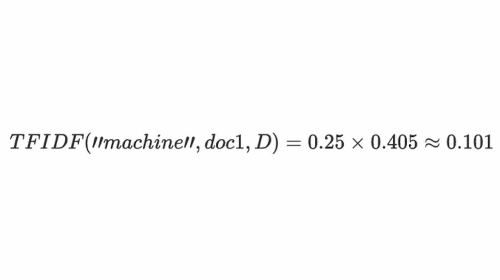
Step 3: Calculate TF-IDF
Increase TF and IDF by: Therefore, “machine” in Document 1 has a TF-IDF score of 0.044.

Practical Example in Python
The scikit-learn library’s TfidfVectorizer is used to implement the TF-IDF idea in Python. A detailed tutorial on TF-IDF implementation and Linear text classification is provided below.
Walkthrough of the Code
Import Required Libraries: To apply machine learning models like Naive Bayes and to perform vectorisation (TF-IDF), require a number of libraries.
from sklearn.feature_extraction.text import TfidfVectorizer
from sklearn.model_selection import train_test_split
from sklearn.naive_bayes import MultinomialNB
from sklearn.metrics import accuracy_score, classification_report
Sample data (replace with your own dataset)
documents = ["This is a positive document.", "Negative sentiment detected.",
"Another positive example.", "Negative review here." ]
labels = [1, 0, 1, 0]  # 1 for positive, 0 for negative
Split the Data: Divide the data into training and testing sets in order to train and evaluate the model. The dataset is automatically divided by the train_test_split algorithm.
X_train, X_test, y_train, y_test = train_test_split(documents, labels,
test_size=0.2, random_state=42)
TF-IDF Vectorization: Next, use TF-IDF to transform the text data into numerical format.
vectorizer = TfidfVectorizer()
X_train_tfidf = vectorizer.fit_transform(X_train)
X_test_tfidf = vectorizer.transform(X_test)- The model learns the vocabulary and performs the TF-IDF transformation when fit_transform is applied to the training data.
- Using the same vocabulary acquired from the training data, transform is performed to the test data.
Train the Naive Bayes Classifier: I’m using the Multinomial Naive Bayes algorithm, which is frequently used for Linear text classification. You can train any classifier you like, including logistic regression, SVM, MLP, etc.
classifier = MultinomialNB()
classifier.fit(X_train_tfidf, y_train)
Make Predictions: Utilise the model to forecast the test data’s labels following training.
predictions = classifier.predict(X_test_tfidf)Evaluate the Model: To determine how well the classifier performed, use the accuracy score and classification report to assess the model’s performance.
accuracy = accuracy_score(y_test, predictions)
report = classification_report(y_test, predictions)
print(f"Accuracy: {accuracy:.2f}") print("Classification Report:\n", report)
Practical Example Summary
from sklearn.feature_extraction.text import TfidfVectorizer
from sklearn.model_selection import train_test_split
from sklearn.naive_bayes import MultinomialNB
from sklearn.metrics import accuracy_score, classification_report

# Sample data
documents = [
    "This is a positive document.",
    "Negative sentiment detected.",
    "Another positive example.",
    "Negative review here."
]
labels = [1, 0, 1, 0]  # 1 for positive, 0 for negative

# Split the data into training and testing sets
X_train, X_test, y_train, y_test = train_test_split(documents, labels, test_size=0.2, random_state=42)

# TF-IDF Vectorization
vectorizer = TfidfVectorizer()
X_train_tfidf = vectorizer.fit_transform(X_train)
X_test_tfidf = vectorizer.transform(X_test)

# Train the Naive Bayes Classifier
classifier = MultinomialNB()
classifier.fit(X_train_tfidf, y_train)

# Make predictions
predictions = classifier.predict(X_test_tfidf)

# Evaluate the classifier
accuracy = accuracy_score(y_test, predictions)
report = classification_report(y_test, predictions)
print(f"Accuracy: {accuracy:.2f}")
print("Classification Report:\n", report)