A potent and increasingly well-liked method for deciphering intricate machine learning models, especially Large Language Models (LLMs), is the use of Sparse Autoencoders (SAEs).
What are Sparse AutoEncoders?
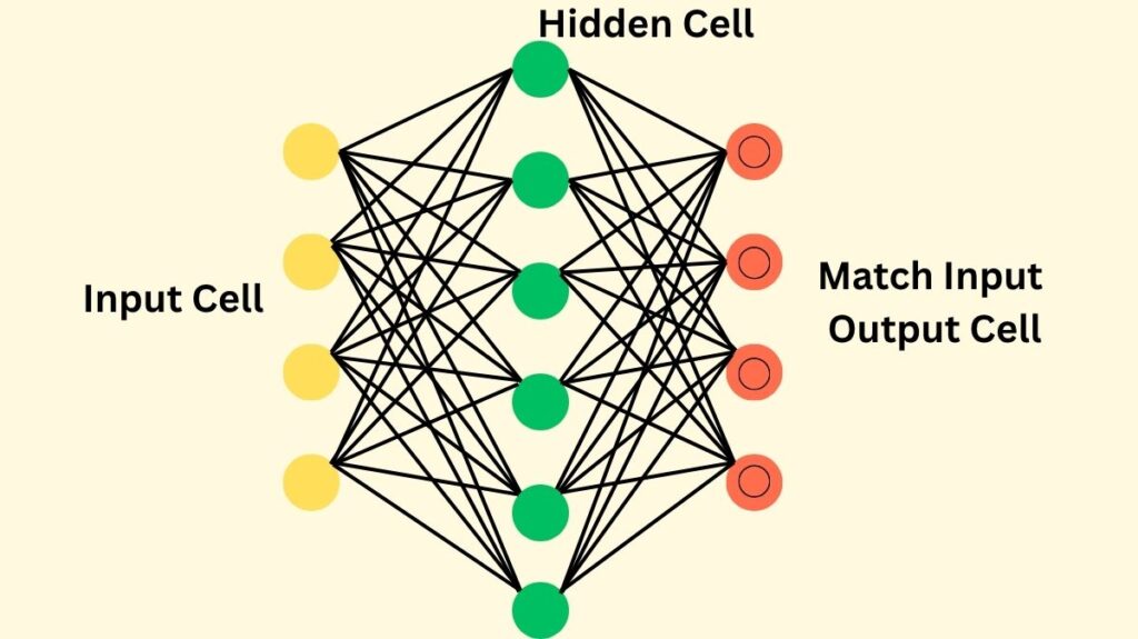
A specific type of neural network intended for feature learning and dimensionality reduction is called a Sparse Autoencoder (SAE). Its main objective is to compress incoming data into an encoded form and then reconstruct it, just like a typical autoencoder. But during training, SAEs impose an important sparsity penalty or limitation. Because of this restriction, the “hidden layer” (also known as the intermediate representation) is encouraged to be sparse, with only a small percentage of its components (neurons or features) being active or non-zero. This approach extends the model beyond basic input replication, challenging it to focus on identifying the most significant and pertinent features from the input data.
History
Although sparse dictionary learning has been there since 1997, sparse autoencoders have lately become more well-known because to its use in improving the interpretability of LLMs and machine learning models. The sparse coding concept in neuroscience served as the impetus for SAEs. This method tackles the difficulty of comprehending how “black box” models, such as LLMs, carry out their intricate functions.
Also Read About Feedforward networks in Neural Network and its Types
Sparse autoencoder architecture

With the addition of a sparsity constraint, an SAE is constructed similarly to a standard autoencoder. A loss function, a decoder, and an encoder make up its three primary parts.
The input data is converted into an intermediate, encoded representation by the encoder. The dimension of this intermediate vector may be more, equal, or less than that of the input. This dimension is usually greater than the input dimension for LLMs. A 12,288-dimensional input for a GPT-3 activation, for instance, might be enlarged into a 49,512-dimensional encoded representation.
Using this encoded form, the decoder then makes an effort to recreate the initial input data. Because of the intrinsic compression and sparsity restrictions, the reconstruction is typically not flawless.
A matrix multiplication, a ReLU activation, and then another matrix multiplication are frequently steps in the process. The encoder matrix is the first matrix, and the decoder matrix is the second. In order to help ensure sparsity, the encoded representation is frequently subjected to a ReLU activation function, which sets any negative input to zero. Tanh or sigmoid activation functions may also be used in older versions or universal autoencoders.
How it Works

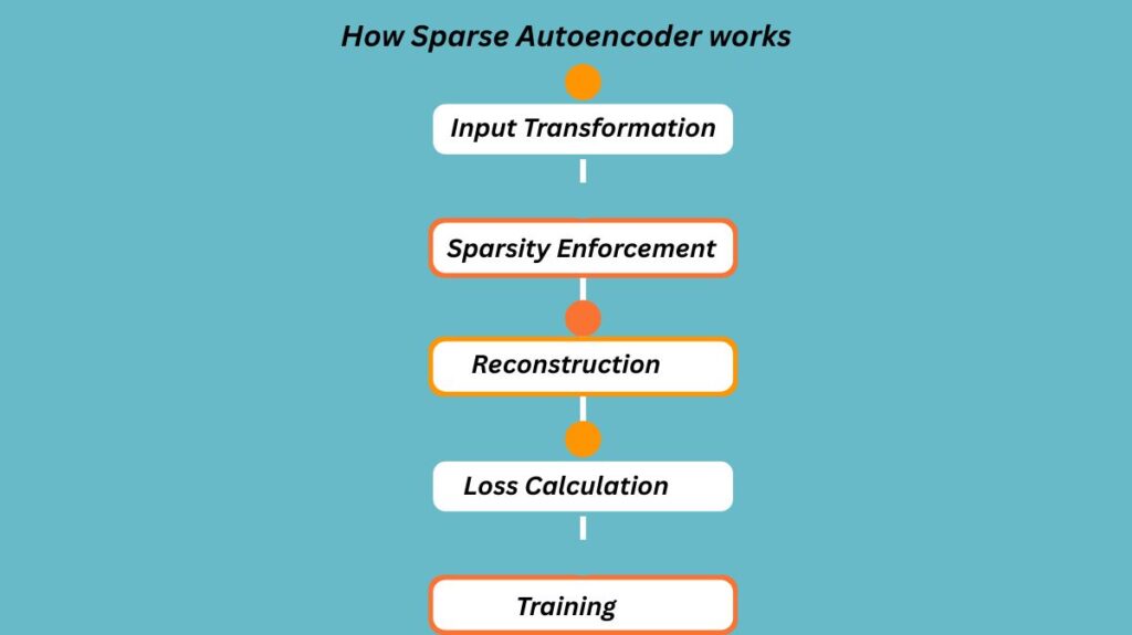
A Sparse Autoencoder’s operational flow consists of the following crucial steps:
- Input Transformation: The encoder transforms the input vector into an intermediate, encoded vector after it has been passed through.
- Sparsity Enforcement: The training loss is increased by a sparsity penalty. Because of this penalty, the SAE is more likely to produce a sparse intermediate vector, which means that very few of its members will be non-zero. KL Divergence, which measures the amount that average hidden neuron activation deviates from a desired sparsity level, and L1 regularization, which penalizes absolute weight values, are common techniques for enforcing sparsity.
- Reconstruction: The decoder tries to recover the original input after receiving the sparsely encoded representation.
- Loss Calculation: The reconstruction error, or the degree to which the reconstructed output deviates from the original input, is combined with the sparsity penalty in the loss function. The L1 coefficient, a critical hyperparameter, establishes the trade-off between preserving reconstruction accuracy and attaining sparsity.
- Training: During training, weights are usually initialized, a forward pass is made, the loss is calculated, and the weights and biases are subsequently updated by backpropagation.
- Application to LLMs: SAEs are trained on intermediate activations that take place both within and between neural network layers when they are used with LLMs. Separate SAEs may be trained for distinct locations or outputs of different layers to analyze the data contained inside a multi-layer model such as GPT-3. It should be noted that SAEs are not specifically optimized for interpretability; rather, optimizing for reconstruction accuracy and sparsity leads to the emergence of interpretable features.
Advantages
Sparse autoencoders have a number of important advantages.
Feature Learning
From vast amounts of unlabelled data, they may extract valuable, high-level features that can be applied to tasks like regression or classification.
Efficiency
SAEs can result in lower processing costs by learning effective representations with fewer active neurons.
Interpretability
Usually, the sparsity constraint results in the identification of more interpretable characteristics, which aids in comprehending the data’s underlying structure and the workings of LLMs. By recognizing particular orientations in activation space that correlate to different features, they can resolve superposition, a phenomenon in which many notions are represented by combinations of neurons.
Robustness
Compared to conventional autoencoders, SAEs may be more resilient to noise and overfitting due to the regularization impact that sparsity provides.
Model Analysis and Steering
Unsupervised techniques for identifying “steering vectors” that can be utilized to regulate or impact model behavior are made possible by SAEs. For instance, Claude mentioned the Golden Gate Bridge in each response when a particular SAE decoder vector was added to its activations. Additionally, they facilitate the identification of circuits in language models, which may enable the elimination of undesired biases.
Proof of Meaningful Learning
Although SAEs were taught just on reconstruction and sparsity, their ability to identify interpretable characteristics indicates that LLMs are picking up meaningful concepts rather than merely memorization of statistics. “MRI for ML models” is the initial step that they are considered to be.
Also Read About Boltzmann Machine Neural Networks Architecture And Types
Challenges with Sparse Autoencoder Evaluations
Sparse autoencoder evaluation poses a number of challenges despite their potential:
Subjective Interpretability
At the moment, assessments are mostly based on human “gut reactions” to the interpretability of the activation inputs for features. Natural language interpretability has no quantifiable underlying ground truth.
Proxy measures
When substituting SAE reconstructions for the original activations, researchers employ proxy measures such as Loss Recovered (the additional loss from faulty reconstruction) and L0 (average number of non-zero elements).
Metric Mismatch
Because L0 is not differentiable and Loss Recovered is computationally costly to compute during training, the proxy metrics used for evaluation frequently do not directly match the loss function used during training. The fact that these proxies are merely stand-ins for the actual objective of “how does this model work” adds another layer of mismatch.
Trade-off
Reconstruction accuracy (Loss Recovered) and sparsity (L0) are usually trade-offs; enhancing one could jeopardise the other.
Possibility of Ignoring Concepts
It’s possible that some crucial ideas in LLMs are difficult to understand, and if interpretability is optimized blindly, this could lead to these ideas being overlooked.
Features
A matching encoder vector and decoder vector define a “feature” in the context of SAEs.
- Identifying the internal concept of the model while reducing interference with other concepts is the function of the encoder vector.
- The “true” feature direction is represented by the decoder vector. In cases when an element of the encoded representation of the SAE is not zero, the associated decoder vector is added to the reconstructed activation after being scaled by the magnitude of that element.
- In other words, linear representations of features in the residual stream space correspond to decoder vectors. These characteristics are often interpretable empirically. The Golden Gate Bridge, neurobiology, well-known tourist destinations, and even particular grammatical constructions like relative clauses are a few examples of concepts that SAEs may identify.
Also Read About What are Deep Convolutional Inverse Graphics Network (DC-IGN)?
Types of Sparse Autoencoder
In order to increase performance, several Sparse Autoencoder implementations and strategies have surfaced, each modifying the sparsity penalty or architecture:
- Vanilla ReLU SAE: A popular and early implementation that is currently regarded as slightly out of date.
- BatchTopK SAE: A more popular method that greatly enhances the trade-off between reconstruction accuracy and sparsity. By keeping only the top ‘k’ activation values and zeroing out the remainder, it replaces the ReLU and sparsity penalty and directly sets the desired sparsity level (a hyperparameter ‘k’).
- TopK SAE: An alternate method that OpenAI discussed that improves the trade-off by altering the sparsity penalty.
- JumpReLU SAE: Another effective substitute strategy.
- Deepmind’s Gated SAE: Adjusts the sparsity penalty to get better reconstruction and sparsity trade-offs.
- Transcoders: A related architecture that attempts to recreate, rather than merely reproduce, the activations of a deep network component given its input. Compared to SAEs, they are said to discover noticeably more interpretable traits.
- Skip transcoders: The addition of an affine skip link to transcoders, known as “skip transcoders,” reduces reconstruction loss without compromising interpretability.
Additional Details
In the area of interpretability, SAEs are thought to be making significant strides. By lowering dimensionality while maintaining crucial characteristics, they are employed for tasks including data compression, anomaly detection (finding outliers based on reconstruction error), and picture denoising. Additionally, they can be used to pretrain deep neural networks, which may help them learn appropriate initial weights and enhance their performance on later supervised learning tasks. Research is still being conducted to solve the difficulties in evaluating SAEs.
Connection to Other Models
Similar to sparse auto-encoders, auto-encoding variational bayes (AEVB) and variational auto-encoders (VAEs) employ an encoder-decoder structure. Neural networks can be employed as probabilistic encoders in AEVB, and the AEVB method is utilized to jointly optimize the parameters. Like autoencoders, the goal function frequently contains an expected negative reconstruction error. VAEs are generative models in which a variational lower limit is optimized by a recognition model (encoder), making approximate posterior inference efficient.
Denoising Auto-Encoders (DAEs): DAEs are a particular type of autoencoder that trains the network to rebuild a clean input from a damaged form, hence expressly enforcing resilience. By compelling the network to infer missing information, this corruption process serves as a regularization, pushing it to learn more significant characteristics. DAEs are related to optimizing the mutual information between the original input and the concealed representation and can be viewed as a method of learning a manifold. DAEs’ training approach “helps to capture interesting structure in the input distribution” and can result in “more useful feature detectors.”
Deep Belief Networks (DBNs): DBNs and sparse auto-encoders are frequently discussed together as unsupervised techniques that build hierarchical layers in a greedy manner. DBNs use the encoder-decoder paradigm, just like Sparse Auto-Encoders, but its building pieces are usually Restricted Boltzmann Machines (RBMs).
Deconvolutional Networks (DNs): DNs expressly lack an encoder, setting them apart from sparse auto-encoders. Rather than seeking to compute features roughly, as some encoder-based methods could, DNs use effective optimization techniques to directly tackle the inference problem (identifying feature map activations).
