What is Deep neural networks?

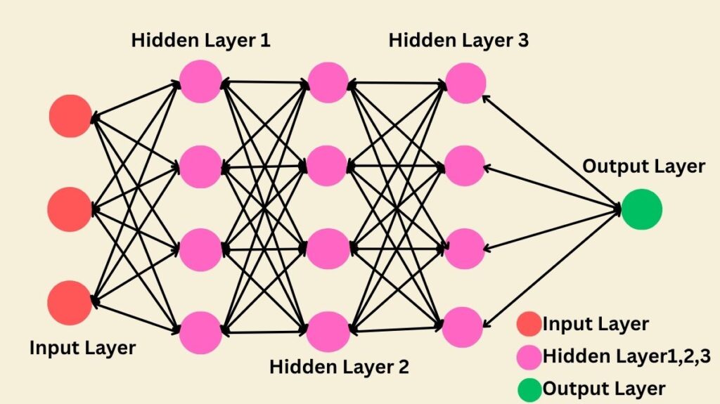
Artificial neural networks having several layers between the input and output are referred to as deep networks, or deep neural networks (DNNs). These networks are the cornerstone of deep learning because of their capacity to extract hierarchical representations and intricate patterns from input.
A deep neural network is a hardware and/or software system that is modelled after the structure and operation of the brain. It is made up of several layers of processing units that operate in parallel to automatically learn data representations. An artificial neural network (ANN) with several hidden layers in between the input and output layers is called a DNN.
To achieve greater levels of data abstraction and complexity, DNNs are more complex versions of traditional neural networks that combine deep architecture with cutting-edge training techniques. The existence of more than three layers, including input and output layers or two or more hidden layers, is referred to as the “deep” aspect. These layers provide the network’s overall output after processing the output from the layer before it.
History of Deep Neural Networks
Neural networks have been around for more than 200 years; their earliest iterations, such as linear networks, were employed for tasks like planetary movement prediction. Important turning points include:
Early Computational Models (1940s-1950s)
In 1943, Walter Pitts and Warren McCulloch put forth a computational model for neural networks that did not learn. D.O. In 1949, Hebb put up the Hebbian learning hypothesis, which was used to the first neural networks. One of the earliest ANNs to be used, the perceptron, was initially described by Frank Rosenblatt in 1958. This caused a lot of public interest and led to more financing. However, development in the United States stalled in the late 1960s because early perceptrons lacked adaptive hidden units and were unable to comprehend exclusive-or circuits.
Deep Learning Breakthroughs (1960s-1970s)
The Group method of data handling (GMDH), which was initially published in the Soviet Union in 1965 and was capable of training arbitrarily deep neural networks, was the first functional deep learning algorithm. The first deep learning multilayer perceptron trained using stochastic gradient descent was published in 1967 by Shun’ichi Amari. Fukushima invented the ReLU activation function in 1969, which is utilized in deep learning.
Backpropagation and CNNs (1970s-1990s)
Seppo Linnainmaa created modern backpropagation in 1970, while David E. Rumelhart et al. popularized neural networks in 1986. Max pooling is a deep learning architecture for CNNs created by Fukushima’s Neocognitron (1979). Yann LeCun et al. created LeNet in 1989 to recognize handwritten ZIP codes.
RNNs (1980s-1990s)
Statistical mechanics (Hopfield network, 1982) and neurology inspired “recurrent” neural networks (RNNs). The Jordan network (1986) and the Elman network (1990) were early, significant works. After the vanishing gradient problem was discovered in 1991, Long Short-Term Memory (LSTM) networks were created and are now the standard option for recurrent neural networks (RNNs) architectures.
Deep Learning Returns
From 2009 to 2012, ANNs outperformed humans in picture identification. ImageNet went to AlexNet (2012) by Krizhevsky, Sutskever, and Hinton. Unsupervised pre-training, GPU processing power, and distributed computing, which enabled larger networks, helped it recover. Since its introduction in 2014, the Generative Adversarial Network (GAN) has emerged as the cutting edge of generative modelling. Large language models like ChatGPT are the result of later advancements in the discipline, particularly in natural language processing, brought about by diffusion models (2015) and the Transformer architecture (2017).
How do Deep neural networks Work?
Deep neural networks use a layered structure to process information.
Structure: An input layer, several hidden (deep) layers, and an output layer are the standard components of a DNN. “Deep” networks are those that include more than three layers, including input and output.
Neurons and Connections: Artificial neurons are the interconnected units or nodes that make up these layers. The strength of the signal is determined by the weight assigned to each neuronal link. Every node has a bias as well.
Processing: The input layer receives input data. After processing signals from other connected neurons, each neuron relays those signals to other neurons. Based on the output of the preceding layer, each layer trains on a distinct collection of features. This input-to-output procedure is called forward propagation.
Activation Functions: Each neuron’s output is calculated by adding the bias and weighted sum of its inputs and using a non-linear activation function. By adding non-linearity to the network, these functions allow it to capture intricate interactions.
Feature Learning: The capacity of DNNs to do automatic feature extraction from unprocessed inputs, sometimes referred to as feature learning, is a significant distinction between them and conventional artificial neural networks (ANNs). Because nodes recombine and learn from elements of earlier levels, the deeper the network, the more complex features the nodes can recognize.
Training (Learning): The process by which the network modifies its weights and biases to increase accuracy is known as training (learning). Typically, it includes:
- Loss/Cost Function: A loss or cost function measures the network’s predicted output versus the true/correct label. Examples include Binary Cross Entropy, MSE, and MAE. Loss reduction is the goal.
- Optimization Algorithms: Optimization algorithms are used to update weights and biases in order to minimize the loss.
The primary algorithm used to decide how much each weight should be altered is backpropagation, which computes the cost function’s gradient. - Gradient Descent: Weights are updated based on the computed gradients using techniques such as Minibatch Gradient Descent, Stochastic Gradient Descent (SGD), Gradient Descent with Momentum, RMSprop, and Adam optimization. The magnitude of the corrective steps is controlled by hyperparameters such as the learning rate.
- The Credit Assignment Path (CAP) is the sequence of changes from input to output in a neural network that elaborates likely causal relationships. The number of hidden layers plus one (for the output layer) equals its depth.
Advantages of deep neural networks

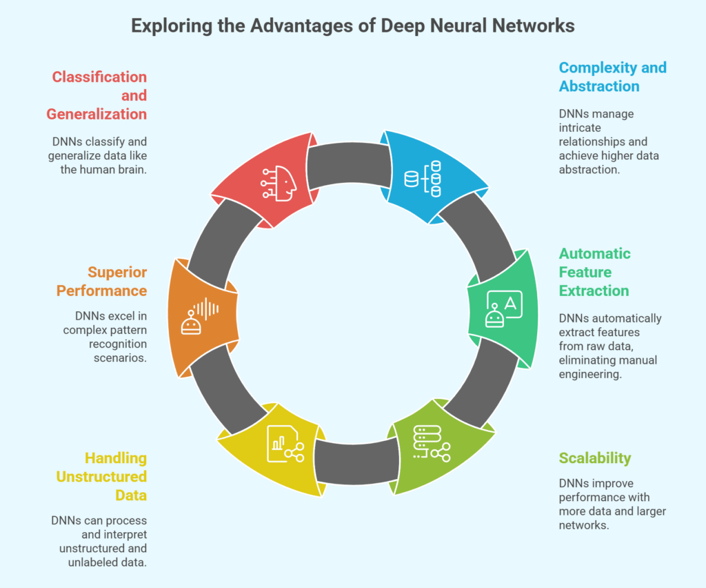
- Greater Complexity and Data Abstraction: Compared to shallow networks, DNNs are able to manage more intricate relationships and achieve higher levels of data abstraction.
- Automatic Feature Extraction: By using a technique called feature learning, they are able to automatically extract features from unprocessed data, doing away with the requirement for human feature engineering.
- Scalability: With more data and larger networks, the DNN architecture enables findings to be fine-tuned. Larger datasets tend to improve their performance.
- Managing Unstructured and Unlabeled Data: One of DNNs’ main advantages is its capacity to handle unstructured and unlabeled data, which makes up the majority of global data, especially in industries like medical. As demonstrated by smart picture albums and bot detection tasks, they are able to group and interpret such data into comparable forms.
- Superior Performance in complicated Scenarios: DNNs perform better than other algorithms in complicated pattern recognition scenarios (like human faces), when simpler techniques like logistic regression classifiers or support vector machines may not be able to identify patterns. They are able to deconstruct intricate patterns into more straightforward ones.
- Classification and Generalization: Just as the human brain can identify images, DNNs can also classify and generalize.
Also Read About What Is Single Layer Perceptron Neural network Architecture
Disadvantages of deep neural networks
Compute-Intensive Training
The process of training DNNs is incredibly computationally demanding and necessitates a major increase in processing power, particularly GPUs. High-performance GPUs can train a deep net in less than a week, whereas fast CPUs may take weeks or months.
Data Requirements
In order to train and attain high performance, DNNs frequently need a lot of labelled data.
Training Challenges
In contemporary deeper networks, conventional backpropagation techniques may result in problems including overfitting and disappearing gradients. The issue of vanishing or exploding gradients might decrease accuracy and lengthen training times.
Complexity and Interpretability (“Black-Box”)
Deep networks are challenging to deal with on a single layer due to their complexity and vast number of training parameters. They are sometimes perceived as “black-boxes” that fail to provide a clear explanation for their forecasts.
Convergence Problems
Depending on the cost function and optimization technique employed, models may not always converge on a single solution because of the presence of saddle points or local minima.
Dataset Bias
The calibre of the training data is essential for DNNs. Poor data may cause the model to learn and perpetuate social prejudices, resulting in unfair results in practice.
Resource Restrictions for Embedded Systems
DNNs’ high memory utility and computational resource requirements, which can result in bandwidth and computational constraints, make their use in embedded systems difficult.
Also Read About What is Perceptron? and Perceptron assumptions
Features of DNNs
- An input layer, several hidden layers, and an output layer make up a multi-layered structure.
- Processing units operate in parallel during parallel processing.
- The ability to automatically learn data representations is known as automatic data representation learning.
- In hierarchical feature learning, more complex features are built at deeper layers by processing the output from the layer before it.
- Non-linear Transformations: To approximate intricate non-linear input-output interactions, use non-linear activation functions.
- Scalability: Made to improve outcomes with larger networks and more data.
- Managing Unstructured Data: Suitable for handling substantial volumes of unlabelled and unstructured data.
- Biology-inspired: Model the composition and operation of the human brain.
DNN types
Although there are many different models in the deep neural network family, Multilayer Perceptrons (MLPs), Convolutional Neural Networks (CNNs), and Recurrent Neural Networks (RNNs) are the three most common varieties.
MLPs, or multilayer perceptrons
The most fundamental kind of deep neural networks are MLPs, which belong to the feedforward artificial neural network family. Each of the completely connected layers that make up this structure applies non-linear functions to a weighted total of all the outputs from the layer before it.
Applications: Multilayer Perceptrons(MLPs) may learn intricate patterns and are best suited for jobs involving organized data with independent characteristics and defined dimensions.
CNNs, or convolutional neural networks
The most prevalent application of Convolutional Neural Networks (CNNs), a unique class of deep neural networks, is in computer vision. They are distinguished by the fact that at least one layer uses convolutions rather than standard matrix multiplication to process input data. Convolutional filters, or kernels, are used by CNNs to extract features from input data, such as pictures. This enables them to record hierarchical or geographic data in high-level forms.
RNNs, or recurrent neural networks
RNNs are intended to handle time-series issues and process sequential data. RNNs differ from other networks in that their node connections create a directed graph along a temporal sequence, which means that both the present and past inputs influence the output at a particular time step. As a result, they have “internal memory” that stores data from earlier calculations.
Applications: Because RNN models can handle data with varying input durations, they are frequently utilized in Natural Language Processing (NLP). They are useful for jobs that require sequential creation or prediction.
DNNs’ challenges
Notwithstanding their remarkable potential, DNNs encounter a number of challenges:
- Computational Burden: With deeper layers, the number of parameters increases explosively, resulting in significant processing loads. Training might demand a lot of resources and sophisticated gear, such as GPUs.
- Vanishing/Explosing Gradients: These issues can arise during training, especially when deeper networks are utilizing conventional backpropagation. They can hinder training and precision.
- Overfitting: DNNs may overfit to the training set and perform badly on invisible data.
- Cross-validation and regularisation reduce this.
- Despite processing unlabelled data, DNNs often need a lot of labelled data to train to function well.
- A DNN is called a “black-box” because of its complex, multi-layered structure, making it difficult for humans to understand how it predicts. Continuous efforts are made to explain AI.
- Dataset Bias: The data that DNNs are trained on influences their learning. The model may pick up on and reinforce societal biases if the data is biassed or unrepresentative, producing unjust or discriminating results.
Applications of deep neural networks

Deep Neural Networks have revolutionized the way complicated tasks are solved in a variety of fields.
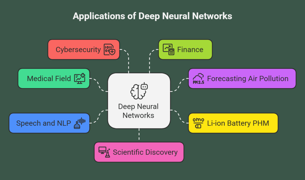
Medical Field
The vast volumes of unstructured and unlabelled data in the medical field are well-suited for processing using DNNs. Their applications include forecasting patient outcomes, speeding up drug discovery, and improving diagnostic accuracy through the interpretation of complex medical imaging.
Forecasting Air Pollution
CNNs, LSTMs, and autoencoders are common and efficient DNN architectures for forecasting air pollution.
Li-ion battery prognostics and health management (PHM)
DNNs are used to forecast the batteries’ state of health (SoH) and remaining usable life (RUL), frequently using voltage, current, and temperature data as input.
Understanding Images and Videos: These are cutting-edge models for comprehending images and videos, including segmenting images, classifying images, and recognising objects. In certain picture recognition tests, they have outperformed human eyesight.
Speech and Natural Language Processing
DNNs are employed in tasks such as sentiment analysis, machine translation, text categorization, speaker identification, and speech-to-text conversion.
Cybersecurity
Used to categorize Android malware, find threat domains, and find URL security threats.
Finance
- By analyzing big financial datasets and identifying intricate patterns, it is used to predict stock market movements and score credit.
- Modelling dynamic systems for identification, control design, and optimization is known as control systems.
- Generational DNNs like GANs and Transformers create new images, music, speech, and literature, even imitating art.
- Self-driving cars need DNNs to identify complicated patterns in real world.
Scientific Discovery
Used to solve partial differential equations in physics and forecast material properties in materials science. Because of their ability to handle complicated, high-dimensional, and frequently unstructured data and learn deep features, DNNs are essentially a potent type of machine learning models.
