Training generative models is the main application for the potent technique known as Auto-Encoding Variational Bayes (AEVB). It tackles the difficulty of carrying out effective learning and inference in probabilistic models, particularly when working with huge datasets and continuous latent variables that have intractable posterior distributions.
What is Auto-Encoding Variational Bayes?
For directed probabilistic models, AEVB is a stochastic variational inference and learning algorithm. Its major goal is to approximate the intractable posterior distribution p(z|x) with a more controlled variational distribution q(z|x). To maximise a variational lower bound on likelihood, the Kullback-Leibler (KL) divergence between the variational and true posteriors is minimized. The reparameterization method, which permits backpropagation over stochastic nodes, is a crucial component that makes this optimization possible. To produce data and learn a latent representation, the technique can be thought of as training a variational autoencoder (VAE).

History
Max Welling and Diederik P. Kingma introduced the “Auto-Encoding Variational Bayes” technique. They presented the concept at the 2014 International Conference on Learning Representations (ICLR) after submitting a paper on the subject in December 2013. This work extends and connects to previous work in fields such as deep generative models, autoencoders, and stochastic variational inference. Around the same time, Danilo Jimenez Rezende, Shakir Mohamed, and Daan Wierstra published another independent study that used the reparameterization approach to draw a similar link between autoencoders, directed probabilistic models, and stochastic variational inference.
Architecture of Variational Autoencoder
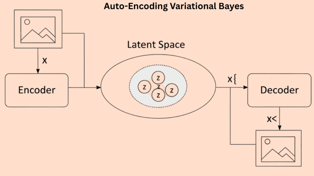
The Variational Autoencoder (VAE) model is frequently used as an example of AEVB. The architecture includes:
Latent Representation (z)
A continuous random variable that is not observed but contributes to the data generation. One way to think about this latent space is as a latent representation or coding.
Prior over Latent Representation p(z)
The distribution from which latent variables are sampled is defined by the prior over latent representation, p(z). A cantered isotropic multivariate Gaussian (e.g., N(0, I)) is a popular option.
Probabilistic Decoder (p(x|z))
The generative model, also known as the probabilistic decoder (p(x|z)), takes a latent code ‘z’ and generates a distribution over the potential corresponding values of the observed data ‘x’. A neural network (such as a multi-layered perceptron, or MLP) is frequently used to accomplish this. It calculates the parameters of the data distribution from ‘z’, such as the mean and standard deviation for a Gaussian or the probabilities for a Bernoulli.
Probabilistic Encoder (q(z|x))
It approximates the intractable true posterior distribution p(z|x) and is also referred to as the recognition model or approximate inference model. It generates a distribution (such as a Gaussian) over the range of values of the latent code ‘z’ that may have produced a data point ‘x’. Additionally, a neural network (such as an MLP) is commonly used to compute the parameters (such as mean and standard deviation) of the variational distribution from ‘x’. Together with the generative model parameters (θ), the encoder’s parameters (φ) are also learnt.
How it Works
The AEVB approach addresses the difficulties associated with learning and inference in intricate probabilistic models:
Variational Lower limit (ELBO): Maximum variational lower limit (L) on the log-likelihood of the data is the main goal of the learning process. Two essential phrases can be used to express this lower bound:
- Regularizer: The KL divergence between the prior distribution p(z) and the variational distribution q(z|x) is measured by this term. This term effectively regularizes the latent space by preventing the approximate posterior from deviating too far from the prior.
- Reconstruction Error: Often read as a negative reconstruction error, this phrase denotes the expected log-likelihood of the data given the latent variables. From its latent representation, the model attempts to recover the input data.
The Reparameterization Trick: This crucial invention makes it possible to optimize the lower bound using conventional gradient descent techniques by allowing backpropagation across stochastic nodes. A deterministic function g of the input x, the variational parameters φ, and an auxiliary independent noise variable ε are used to generate a sample z rather than sampling directly from the variational distribution q(z|x). This allows for the efficient computation of gradients by making the sampling procedure differentiable with respect to φ.
Algorithm: The AEVB method usually employs a minibatch technique for parameter changes and is intended for online, non-stationary environments. Stochastic gradient ascent is used to iteratively update the parameters (δ for the variational model and θ for the generative model) after they are initially initialized randomly. By differentiating the stochastic estimator of the lower bound (SGVB estimator), the gradients are calculated.
Advantages of AEVB
AEVB provides a number of noteworthy advantages:
Effective Inference and Learning: It offers a quick training process that approximates the posterior and marginal likelihoods and estimates parameters for data production.
Scalability: The approach is appropriate for contemporary machine learning applications since it can scale to big datasets.
Handles Intractability: Even in cases when posterior distributions are unmanageable, it functions well.
Produces Realistic Samples: Tests have demonstrated that it is capable of producing realistic samples, including Frey Face pictures and MNIST digits.
Outperforms Other Methods: It has been demonstrated to perform better than other online learning techniques, such as the Wake-Sleep algorithm on held-out likelihood, achieving better results and a significantly faster convergence.
Learns Latent Representations: For tasks like coding, data representation, denoising, and visualization, it automatically picks up a latent representation of the data.
Inherent Regularization: Often, the variational bound eliminates the requirement for nuisance regularization hyperparameters by providing a regularization term that promotes the approximate posterior to be near the prior.
Resistance to Overfitting: It’s interesting to note that the approach seems to be resistant to the quantity of latent variables; the regularizing impact of the lower bound prevents overfitting from occurring when extraneous latent variables are included.
Also Read About Boltzmann Machine Neural Networks Architecture And Types
Disadvantages/Challenges
AEVB and VAEs have significant drawbacks and difficulties in spite of their advantages:
Bias in Decision-Making
When making decisions, practitioners frequently substitute the variational distribution for the posterior, which can result in inaccurate estimations of the expected risk and bad choices. This is because the model itself might not exactly match the distribution of the underlying data, and the variational distribution might not exactly equal the posterior distribution under the fitted model.
Underestimation of Variance
VAEs are known to systematically underestimate variance in the variational distribution they recover (which minimizes the reverse KL divergence), which makes them an unsuitable option for importance sampling proposal distributions in certain situations.
Model vs. Data Mismatch
The model that the VAE learns may not accurately reflect the actual data-generating process, even when posterior expectations are computed accurately.
Overconfidence
The vanilla VAE’s performance in classification tasks may suffer if it becomes overconfident in its posterior predictive density.
Posterior Collapse
A recognized failure scenario in which the conditional probability is independent of the latent variables and the variational distribution is equal to the prior. Even though there are ways to lessen this, AEVB variations might still perform better.
The cost of computation while making decisions
Fitting numerous VAEs is necessary for advanced decision-making processes, like the suggested three-step method utilising multiple importance sampling. This adds computing cost in comparison to a standard VAE.
Model Quality Check Difficulty
Neural networks employed in VAE-style architectures are black-boxes, which can make it challenging to determine the model fit’s quality, particularly in mission-critical applications where worst-case performance is essential.
Features
AEVB offers a framework with a number of noteworthy features:
- Training generative models that can generate fresh data samples that resemble the training data is the purpose of generative modelling.
- Latent Space Learning: This technique is helpful for applications like data compression and visualization because it learns a meaningful low-dimensional latent representation (or code) of the data.
- Probabilistic Encoder/Decoder: By training a probabilistic encoder (recognition model) and a probabilistic decoder (generative model), it clearly connects to autoencoders.
- Estimating the Marginal probability: This method can give a rough estimate of the marginal probability for assessing a model.
- Stochastic Optimization: For effective optimization on big datasets, stochastic gradient techniques are used.
- Image generation (MNIST, Frey Face datasets), image denoising, inpainting, and super-resolution, novelty detection in control applications, mutation-effect prediction for genomic sequences, and Bayesian hypothesis testing for single-cell RNA sequencing data (scRNA-seq) are just a few of the domains in which it has been used.
Also Read About What is Hierarchical composition, How it works, and features
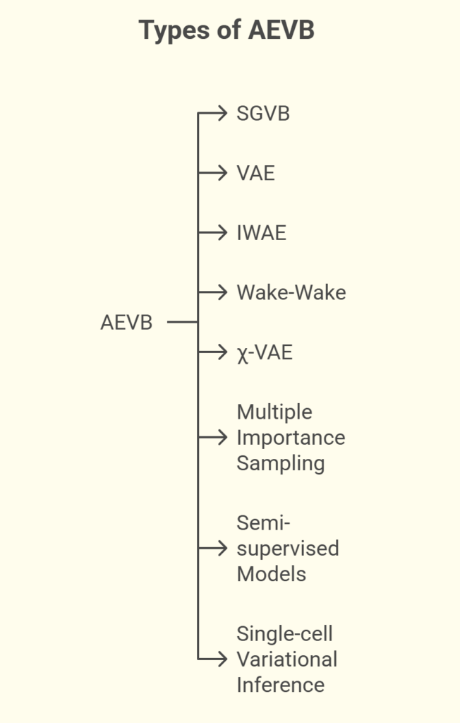
Types of AEVB

Due to AEVB’s success, numerous extensions and associated techniques have been developed:
SGVB (Stochastic Gradient Variational Bayes)
The generic estimator of the variational lower limit proposed by Kingma and Welling, which AEVB particularly applies to i.i.d. datasets with continuous latent variables per datapoint, is called stochastic gradient variational bayes, or SGVB.
Variational Autoencoder (VAE)
This is the standard model example that maximizes the lower limit using the AEVB process; its encoder and decoder are usually neural networks.
Importance Weighted Autoencoders (IWAE)
This variation is based on importance sampling estimates and employs a stricter lower constraint on the evidence (IWELBO). When estimating posterior expectations, IWAE empirically frequently performs better than VAE.
Wake-Wake (WW)
Similarly to AEVB, Wake-Wake (WW) is an inference process that uses a recognition model, but its goal is different: it looks for a variational distribution that minimizes the forward KL divergence.
χ-VAE
An innovative version of the WW algorithm that fits the variational distribution by minimizing the χ² divergence, which has advantageous characteristics for fitting a proposal distribution.
Multiple Importance Sampling (MIS)
A decision-making method that improves estimates for complex posteriors by combining many approximation posteriors as proposal distributions.
Semi-supervised Models
The M1+M2 model, which uses discrete latent variables for class information, is one example of a semi-supervised learning environment where AEVB principles can be applied.
Single-cell Variational Inference (scVI)
One particular use of hierarchical Bayesian modelling with VAEs for examining single-cell RNA sequencing data is called single-cell variational inference (scVI).
More Information
Results from experiments show that AEVB is effective.
Performance measures: AEVB performs better than alternative techniques on held-out likelihood measures and produces realistic samples. On datasets like MNIST and Frey Face, it demonstrates noticeably faster convergence and superior results when compared to the Wake-Sleep technique.
Latent Space Visualization: The learnt encoders (recognition models) enable the visualization of high-dimensional data projected onto a low-dimensional manifold for low-dimensional latent spaces (e.g., 2D), exposing structures such as digit manifolds in MNIST.
Implications for Decision-Making:
- Biassed estimations and less-than-ideal choices result from directly substituting the variational distribution for the posterior.
- According to theoretical findings, a posterior approximation that is different from the variational distribution used for model fitting ought to be utilized for sound decision-making.
- Since it helps regulate sample efficiency, overestimating the posterior variance is frequently preferable to underestimating it in the context of importance sampling.
- One important realization is that the best proposal distribution for decision-making may not be the same as that for model learning.
- It has been demonstrated that a three-step process (fitting a model, fitting multiple approximation posteriors, and then integrating them via multiple significance sampling) outperforms the state-of-the-art in demanding applications such as the processing of data from single-cell RNA sequencing. In FDR estimation, this process greatly enhances measures such as mean absolute error.
- The suggested three-step decision-making process still performs better than methods like cyclical annealing and lagged inference networks, even if they can enhance VAE performance by reducing posterior collapse.
Also Read About Stochastic Gradient Variational Bayes and its Advantages
