Shortest Path in Algorithm

In graph theory, shortest path in algorithm estimation algorithms are essential, particularly for weighted graphs with edges that have associated costs or distances. Finding a path between two vertices that minimises the sum of the edge weights is the goal. This total amount is known as the path’s weight or length. The shortest path in algorithm may not be clearly defined if a graph has a cycle with a negative total weight because it is possible to go through the negative cycle indefinitely in order to arrive at an arbitrarily low negative cost. To avoid such problems, the techniques given here assume non-negative edge weights.
Dijkstra’s Algorithm
Dijkstra’s Algorithm is famous for finding the shortest path in algorithm from a beginning vertex to all reachable vertex. The Dijkstra Method Dijkstra’s greedy method resembles weighted Breadth-First Search. A “cloud” of vertices is iteratively expanded, with new vertices added in ascending order of their shortest distance from the originating vertex. D[v], the currently best-known distance between s and vertex v, is tracked by the method. D[s] is initially set to 0 and D[v] to ∞ (infinity) for any vertex v ≠ s. Starting empty, C symbolises the “cloud” of vertices with the shortest path.
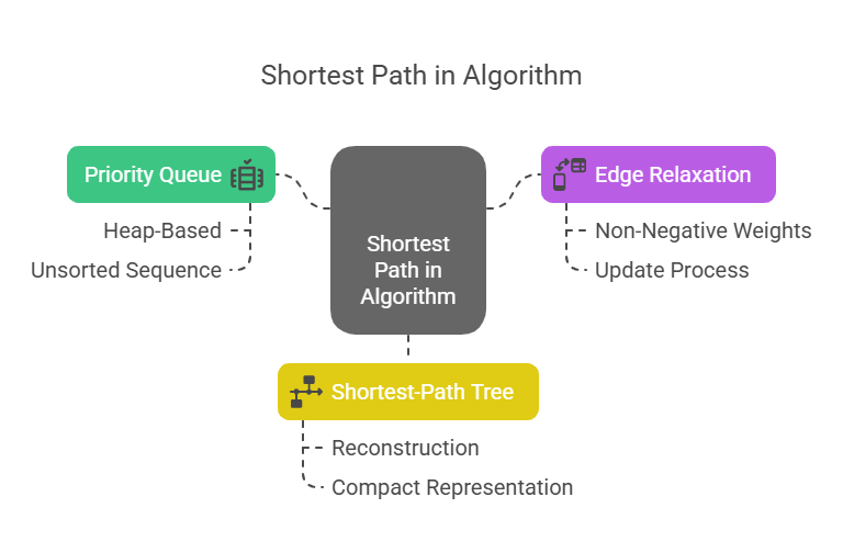
The method chooses a non-C vertex u with the lowest D[u] label per iteration. The cloud C is then “pulled” into this vertex, u. The algorithm modifies the D[v] labels for each of u’s neighbours v that are remaining outside of C after u is added to C. We refer to this update process as edge relaxation.
If D[u] + w(u,v) < D[v], then D[v] is the relaxation process for edge (u,v). If u shortens the path to v, D[v] is adjusted to reflect the lesser distance.
The method terminates when all vertices outside the cloud or inaccessible are gone. The correct shortest path in algorithm length from s to u is stored in the D[u] label of a vertex u when it is pulled into C. The non-negativity of edge weights is necessary for this accuracy.
Running Time Analysis
The data structures employed affect Dijkstra’s algorithm’s performance, especially for the priority queue Q, which efficiently selects the least D[u] label by storing vertices outside the cloud.
The algorithm includes:
- Q has n insertions, one per every vertex.
- For every vertex pushed into the cloud, Q receives n calls to remove min().
- m (one for each edge relaxation, in the worst scenario) calls to update() on Q.
Using a heap-based adaptable priority queue: O(log n) time is required for each operation (insertion, remove min, update). O((n + m) log n) is the overall running time as a result. It reduces to O(m log n) for a linked network where m ≥ n-1.
Using an unsorted sequence as a priority queue: On an unsorted priority queue, remove min requires O(n) time, whereas location-aware entries allow key changes in O(1). Basic graphs take O(n^2 + m) time to run, decreasing to O(n^2).It is generally desirable to use the heap approach for graphs with fewer edges (m < n^2 / log n).
Implementing the unsorted sequence can be more effective for dense networks (many edges, m > n^2 / log n). An optimal O(m + n log n) time complexity can be attained via a sophisticated data structure such as a Fibonacci heap.
An Example of Python Code The shortest-path distances vertex are calculated in the Python version of Dijkstra’s algorithm that follows. For effective priority queue operations, it makes use of an Adaptable Heap Priority Queue.
Example:
import heapq

class Graph:
    def _init_(self):
        self.adj_list = {}
    def add_edge(self, u, v, weight):

        """Add a directed edge from u to v with a given weight."""
        if u not in self.adj_list:
            self.adj_list[u] = []
        if v not in self.adj_list:
            self.adj_list[v] = []
        self.adj_list[u].append((v, weight))

    def dijkstra(self, start):
        """Find the shortest paths from the start vertex to all other vertices."""
        distances = {vertex: float('inf') for vertex in self.adj_list}
        distances[start] = 0

        priority_queue = [(0, start)]

        while priority_queue:
            current_distance, current_vertex = heapq.heappop(priority_queue)

            # Skip processing if we've already found a shorter path
            if current_distance > distances[current_vertex]:
                continue

            for neighbor, weight in self.adj_list[current_vertex]:
                distance = current_distance + weight

                # If a shorter path is found
                if distance < distances[neighbor]:
                    distances[neighbor] = distance
                    heapq.heappush(priority_queue, (distance, neighbor))

        return distances

# Example Usage
if __name__ == "__main__":
    g = Graph()
    g.add_edge("A", "B", 4)
    g.add_edge("A", "C", 2)
    g.add_edge("B", "C", 5)
    g.add_edge("B", "D", 10)
    g.add_edge("C", "E", 3)
    g.add_edge("E", "D", 4)
    g.add_edge("D", "F", 11)

    start_vertex = "A"
    shortest_paths = g.dijkstra(start_vertex)
    print(f"Shortest paths from vertex {start_vertex}:")
    for vertex, distance in shortest_paths.items():
        print(f"Vertex {vertex}: {distance}")
output:
Shortest paths from vertex A:
Vertex A: 0
Vertex B: 4
Vertex C: 2
Vertex D: 9
Vertex E: 5
Vertex F: 20
Reconstructing the Shortest-Path Tree
Rebuilding the Tree with the Shortest Path in algorithm The pathways themselves are not explicitly provided by shortest path lengths, even though it calculates the shortest distances. A shortest-path tree is made up of the collection of all the shortest pathways. Dijkstra’s d[v] values can reconstruct this tree.
Ensure v ≠ s meets the criterion = d[u] + w(u,v) if u is the preceding vertex on a shortest path in algorithm from s to v. For each incoming edge to v, locate an edge (u,v) that fulfils this equation to discover v’s shortest path in algorithm tree parent. Time to reconstruct is O(n+m). The shortest-path tree compactly represents all shortest paths s.
